Photography: Megapixel Conspiracy

... and a Tamron SP 300mm f/2.8 review

Falk Mielke, University of Antwerp, January 10, 2023

image processing photography demosaicing lens review

(You can download this notebook here.)

Motivation

You might think that I have been writing my PhD thesis this last year. Indeed, I should have. And I did. But maybe I was distracted (a bit) by photography. It’s a great hobby, and one which keeps growing, and on which you keep learning.

This post has three parts: First, I will review a lens which I purchased second hand, the Tamron SP 300mm f/2.8 LD IF.

Second, when using it, I dug into demosaicing of digital images, and why it is that we actually get much fewer megapixels out of a camera than the manufacturers tell us.

And lastly, I then imitate the demosaicing algorithm of cameras and professional photo editing software in a slow and inefficient way (but it works!).

Enjoy reading, but even more, enjoy photography!

Motivation
Lens Review: Tamron SP 300mm f/2.8 LD IF
1. Introduction
2. Strengths
3. Limitations
4. Sample Images
5. Summary
Demosaicing and the Megapixel Conspiracy
A Custom Interpolator
1. Interpolation/Demosaicing Code
2. Discussion
Summary

Lens Review: Tamron SP 300mm f/2.8 LD IF

Introduction

I have been photographing a lot lately. It is a great hobby. And admittedly I have grown a certain equipment addiction. Maja is surely not innocent in fostering this hobby - we take turns to free our backs from the little ones. Yet while Maja turned more to wildlife photography and small birds in particular, I have often been doing the family part. My favourite lenses are, logically, short prime lenses.

But of course I also went for the local wildlife. Sparrows, pidgeons, ducks - you name it! Wandering around with a consumer grade telephoto zoom lens, I recently got annoyed that, compared to the family photos, images are dark or noisy, sharpness is underwhelming.

I figured it must be the aperture and glas, and went down the rabbit hole of telephoto prime lenses.

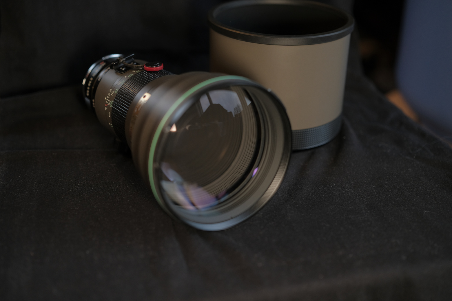
And now, on a great occasion, I purchased this old lady: the Tamron SP 300mm f/2.8 LD IF.

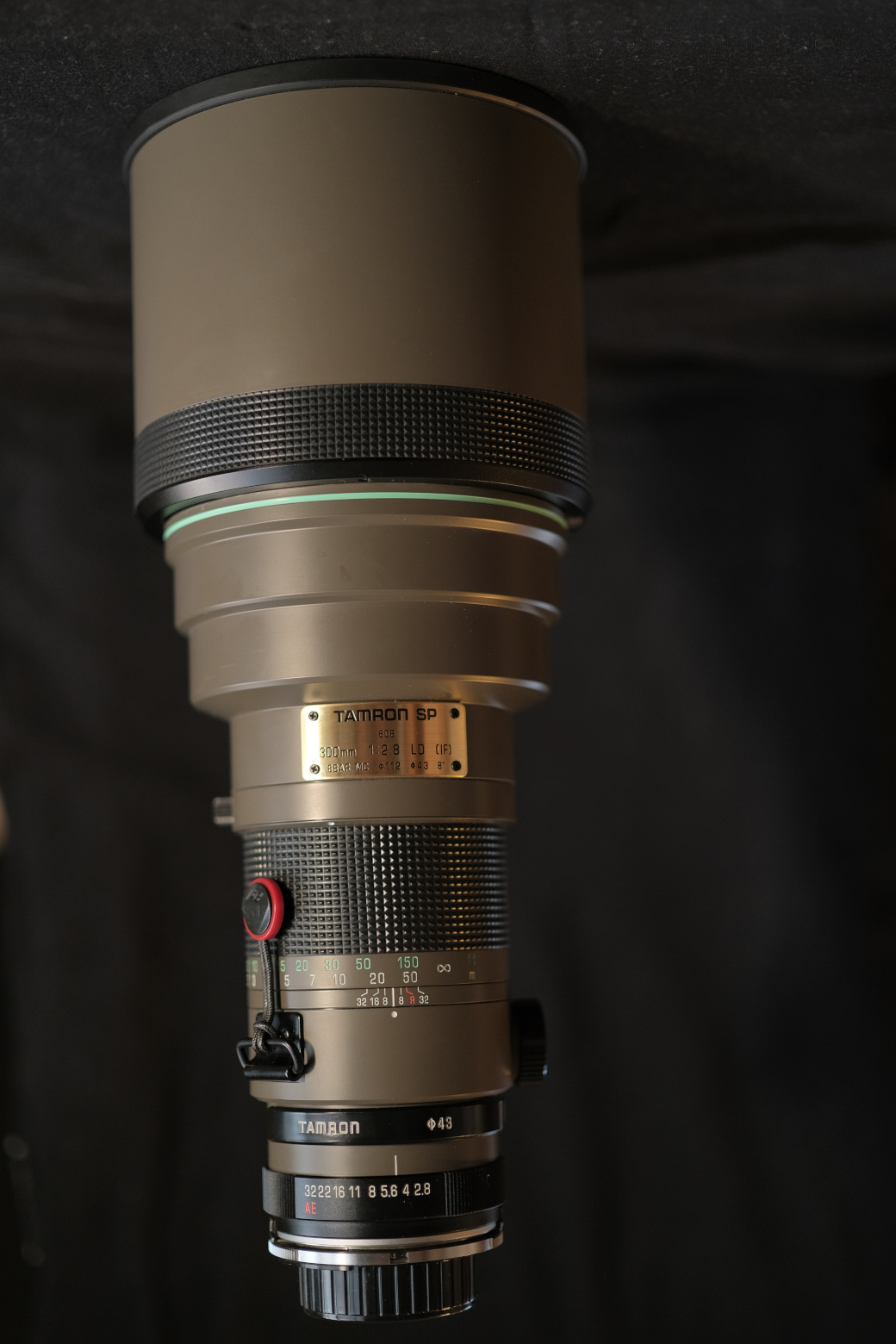
This used to be an expensive, professional piece of equipment, and I figured it would be a great lens to learn on! It is approximately my age, and the seller admitted there were signs of moisture in the inner lens. In consequence, I got it for a humane price (440EUR). After receiving it, I applied some youtube beauty tipps and could not spot the moisture afterwards; the lens is in a great state and ready to be set loose on the local pidgeon population. The maximum aperture of f/2.8 and the sufficient reach (equiv. 450mm on my cropped sensor) are promising. It is built (and colored) like a tank, accordingly heavy and robust (but leaky to wind, dust, and water), all as one would expect. It has a steampunk soul, all manual high-tech.

Yet is it fit for being adapted to a Fujifilm X-T4 camera? There are some reviews online praising it, in general, yet photography is under fast development and I was wondering whether these reviews still count for modern high resolution sensors. Maja once used to have a cheap tamron tele-zoom, and I still cringe at the levels of chromatic aberration it experienced - could the older, but more professional Tamron lens be better? It was also unclear whether a Fujifilm teleconverter would fit behind the adapter. And I was not sure whether manual focus was prohibitive.

So this was a venture.

TL;DR: The lens is fun to use, and one can get great images with it. It is just sufficiently sharp, the depth of field and focal length hold up to their promise, the teleconverter works. Using manual focus is no real obstacle on modern mirrorless cameras. However, strong longitudinal chromatic aberration is an issue in some circumstances.

Sample Images can be found below.

Strengths

All the specs are online: the lens weighs $\approx 2kg$, has no weather sealing, but internal focus, filter inlet, and sits on the “adaptall-2” mount system.

The good news: the lens is reasonably sharp and can produce great images out-of-camera, even with a 26 megapixel sensor.

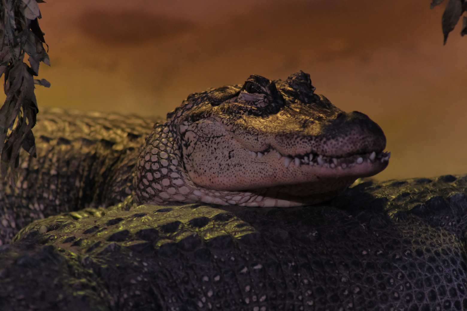Alligator mississippiensis, in bad light. Out-of-camera JPG.

Depth of field wide open is phenomenal. Not only does this give great out-of-focus backgrounds; the wide maximum aperture of course reduces constraints on the other exposure settings!

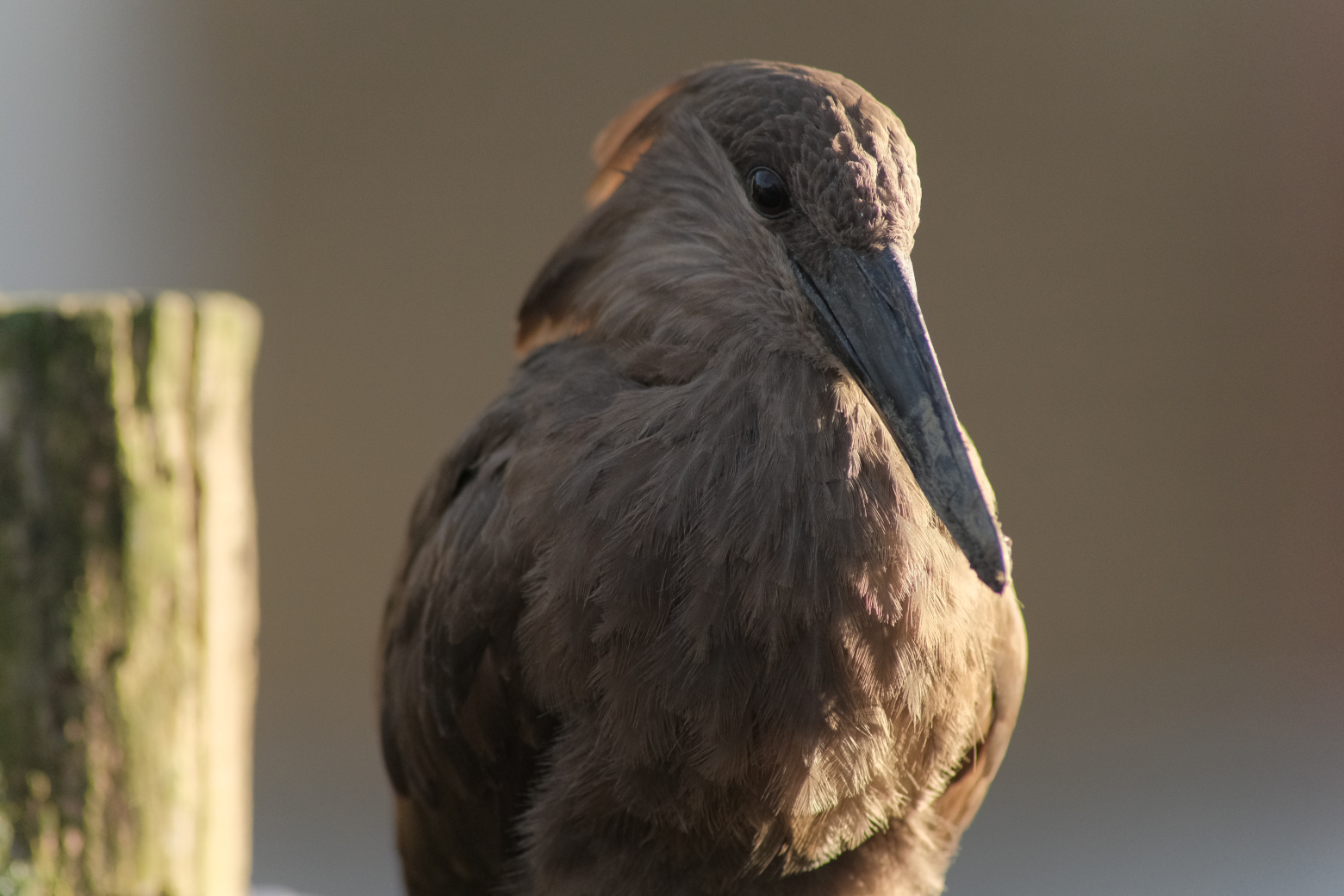Scopus umbretta, at approximately minimum focusing distance ($2.5m$). Out-of-camera JPG.

Whereas I have been mostly shooting “slow shutter to avoid ISO” on my telephoto zoom (pretty dull mode of operation: there is just no choice), I can now play around with shutter speed and aperture at reasonable ISO. Just as one would expect. And this is the great benefit of this lens for me: it is an affordable lens to learn photography on.

Oh, and of course it is great for portraits.

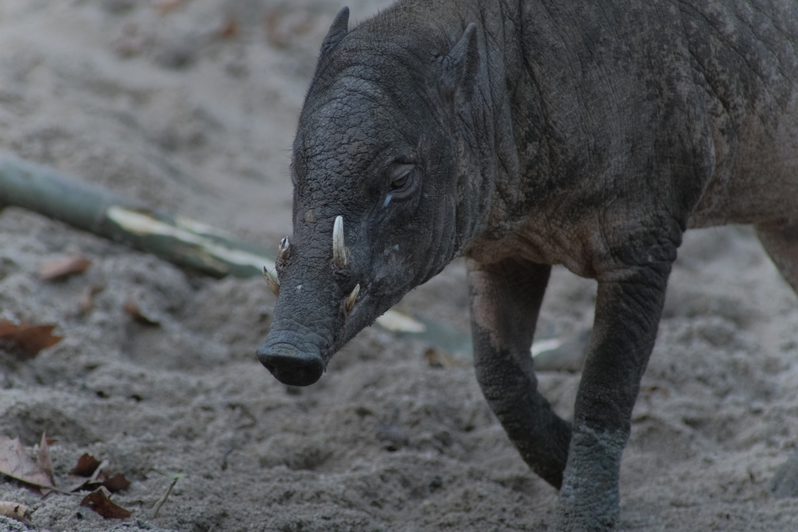Babyrousa celebensis, who else would you want for a portrait shoot? Out-of-camera JPG.

Just as a brief, non-scientific test: the Fujifilm XF1.4x TC WR Teleconverter fits behind the adapter.

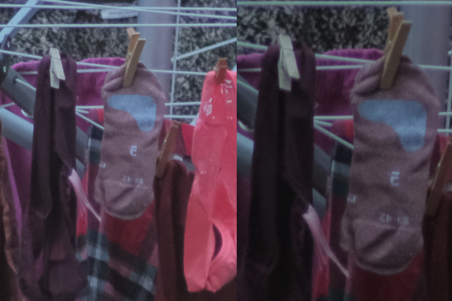If you like close-ups of your neighbours laundry, a teleconverter (right image) might be your thing. Out-of-camera JPG.

Limitations

The Good

The obvious caveat: there were no electronic sensors and controls in the film era. It is all manual, does not even report back the aperture setting. And in consequence, some situations are challenging.

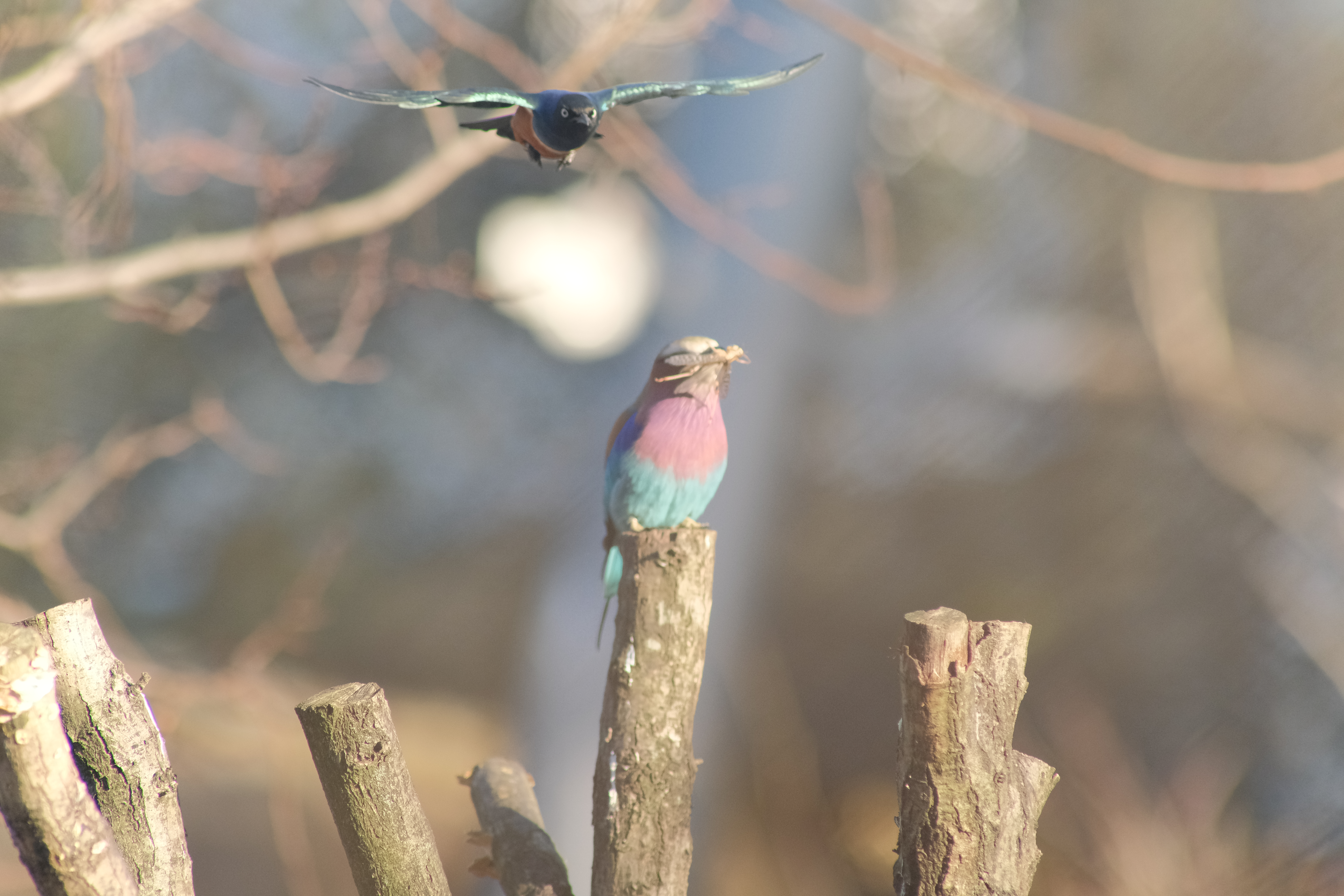Coracias caudata, expecting the approach of Lamprotornis superbus. Photographing birds in flight will be a gamble with manual focus.

The tools to help are focus peaks, and focus peeking, and practice. The first are red marks on sharp edges which can be superimposed on the electronic viewfinder image (mirrorless cameras) during manual focus - check your camera settings. The second is the ability to digitally zoom (“punch”) in on a region of interest (also, only on mirrorless; I got this mapped to my rear dial push). Practice is the only help remaining on a DSLR camera system. Hence, if you are on a mirror, this thing might be much harder to use.

For me, on a mirrorless Fuji, manual focus has always been fun.

Likewise, if you are up for handheld video shooting, this is definitively not the ideal equipment. It is heavy and not stabilized. There is no zoom. The main problem which is aleviated by the Tamron, i.e. ISO noise on lenses with worse maximum aperture, is less a problem in videos where it could be controlled by temporal interpolation. Thus, I would usually prefer a modern zoom lens for handheld video shooting.

The Bad

How could people in the eighties live without nano coating and nanoprecision laser manufacturing? They certainly did not have good zebra photos back then (unless they used monochrome, see below).

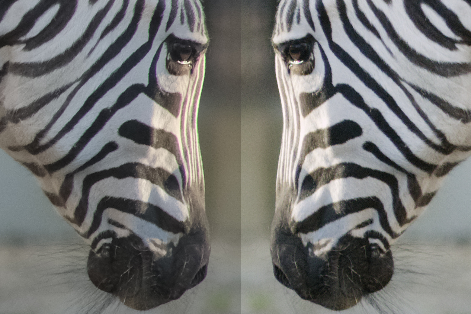Equus zebra - the allegory of chromatic aberration. Left: out-of-camera JPG. Right: after correction.

I had read this review here prior to purchase and can confirm that chromatic aberration is present with this lens on contrasting edges. I can also confirm that it is easy to correct, which I did in RawTherapee.

Yet there is another type of chromatic aberration, which did not go away that easily.

The Ugly

As you can see below, this lens suffers from horrible longitudinal chromatic aberration when photographing “wide open”, i.e. at f/2.8.

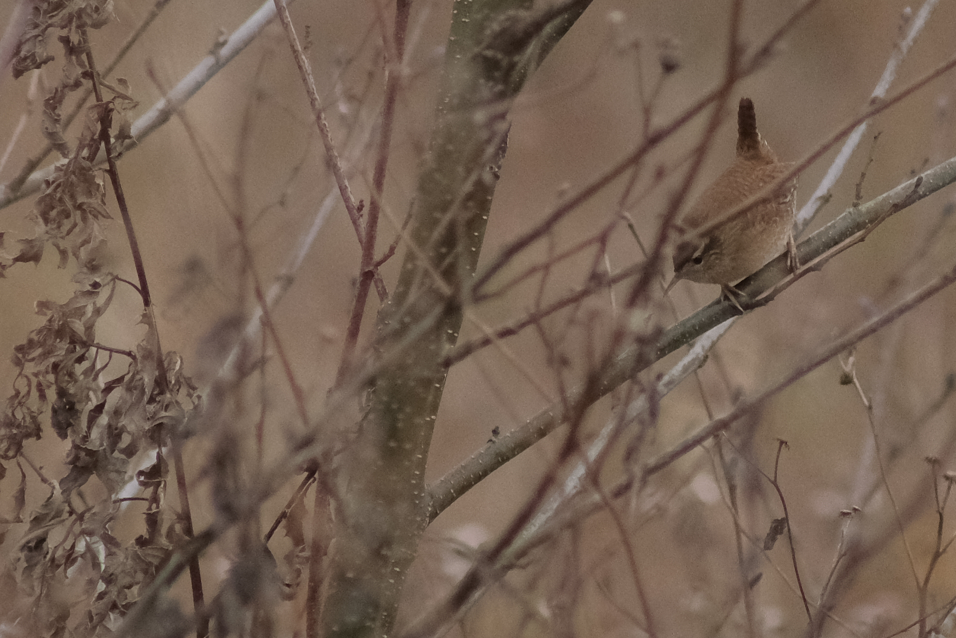
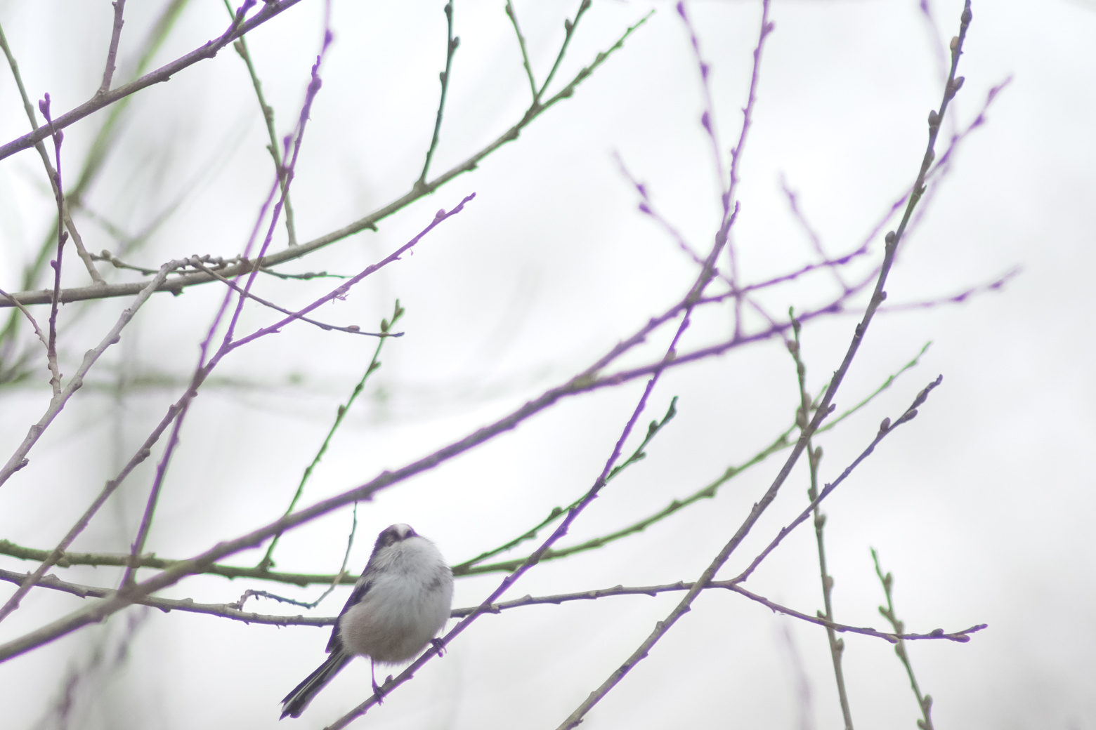Aegithalos caudatus, singing the threnody of longitudinal chromatic aberration. Out-of-camera JPG.

I see three ways about this: (i) Stopping down. Stopping down is not an option. If I would have wanted to photograph at f/5.6, I could have used my previous lens in the first place.

(ii) Avoid contrasting edges. The sky in the background is a sign of poor composition skills, anyways.

(iii) Make the image monochrome. And THIS is where I stumbled upon the greatest conspiracy I ever discovered. Who knows, maybe the greatest conspiracy of all times (except that other one about christmas - ask your parents about it)? I went down the rabbit hole of image demosaicing and sensor layouts. Stay tuned to read below what I found out.

Nevertheless, even the worst longitudinal chroma nightmares still make good black-and-white photos. It dawned on me why so many people online post their high quality digital color photos in monochrome.

Sample Images

Prior to that great conspiracy, your browser will have to process some high quality photos I shot at the Antwerp Zoo. You can download the RAW files and the RawTherapee XMLs, if you like.

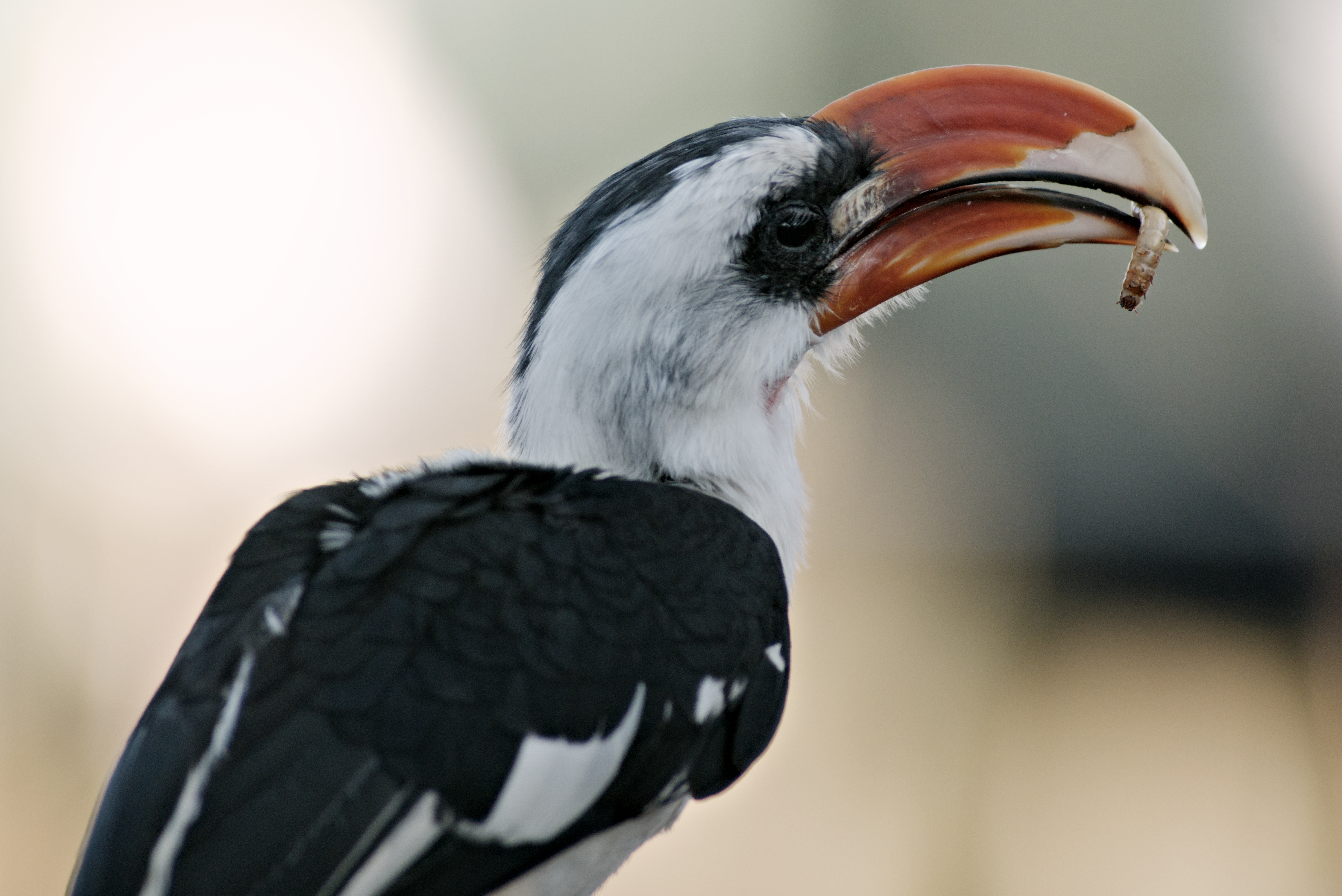Tockus deckeni, with a touch of Classic Chrome: RAW pp3

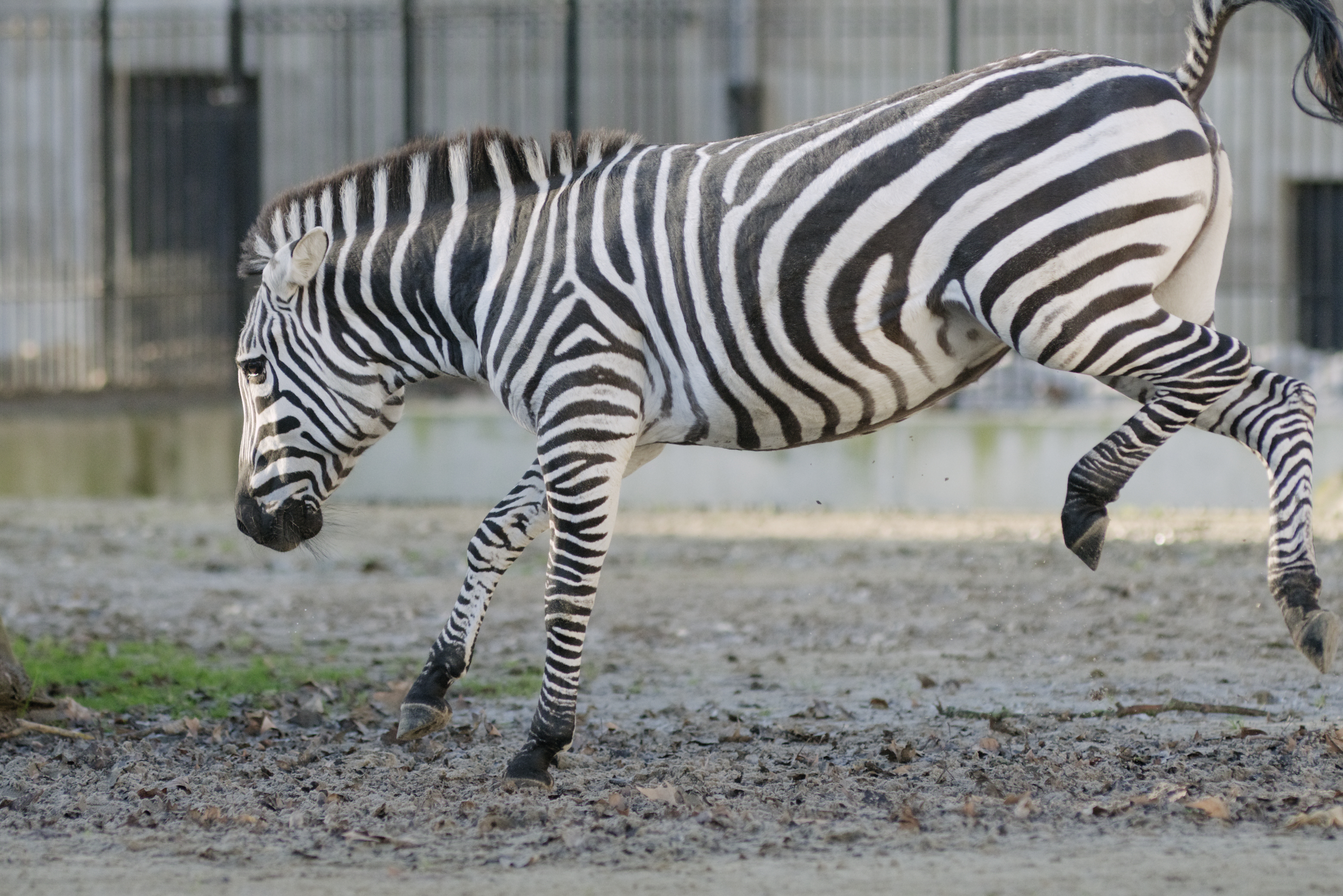Equus zebra, unsuccessfully trying to mock my humble manual focusing skills: RAW pp3

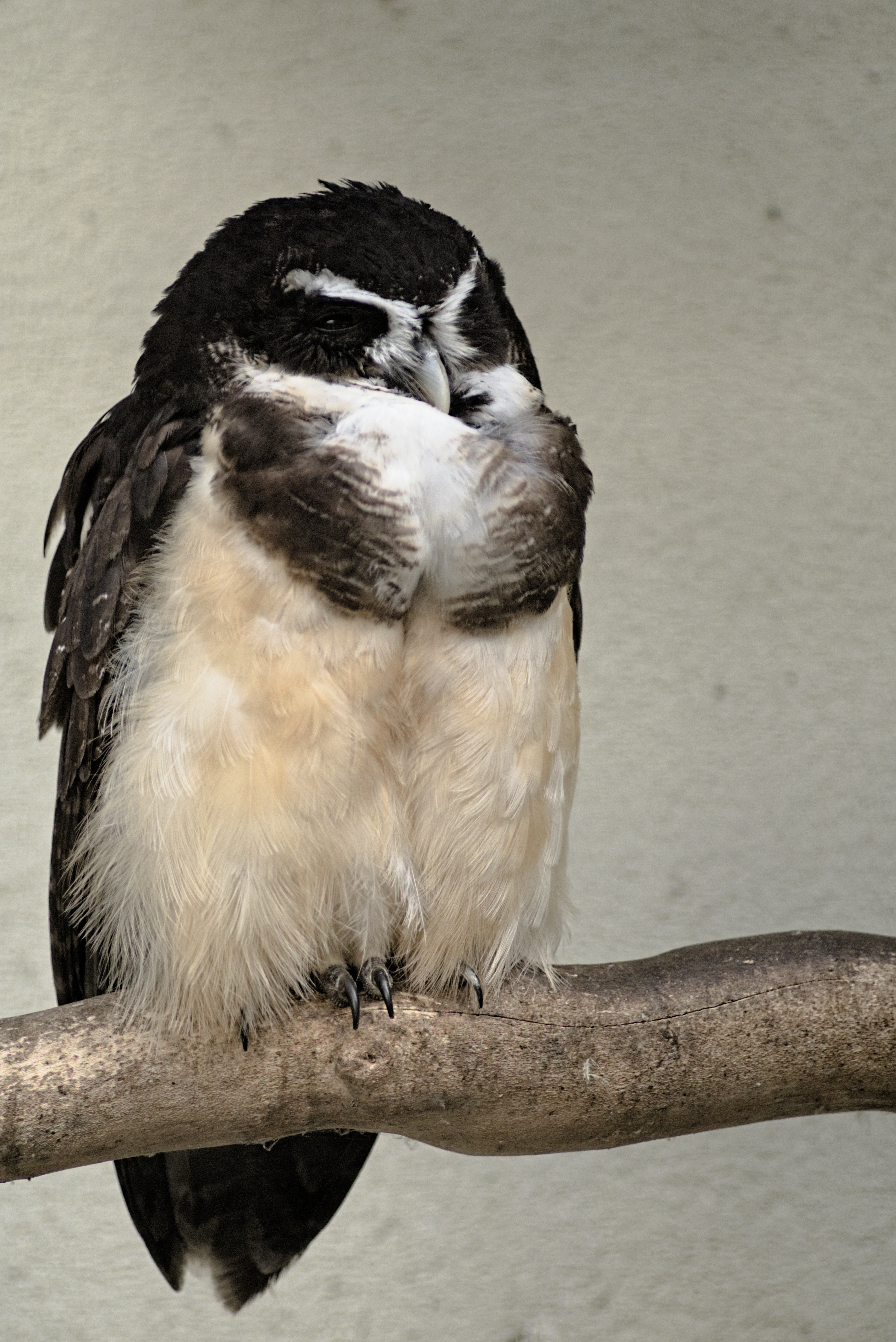Pulsatrix perspicillata, recovered from behind thick cage bars: RAW pp3

Summary

This steampunk lens is a joy to use, and I like the image results. The specs and limitations are expectable. It will benefit from some learning by “rolling up my sleeves” in image post-processing.

Thus, pretty easy to rationalize this idiotic purchase (it’s mostly for pigeons, after all).

Demosaicing and the Megapixel Conspiracy

Mosaic Data

Let us now take a close look at a photo of a wren. (We take a wren because we can, and process it in python then.)

import rawpy as RAW
import imageio as IO
import matplotlib.pyplot as PLT
import numpy as NP
import skimage.exposure as EXP
dpi = 100
fig = PLT.Figure(dpi = dpi, figsize = (5*500/dpi,5*500/dpi))
fig.subplots_adjust(bottom=0, left=0, right=1, top=1)
ax = fig.add_subplot(1,1,1)

path = 'images/wren_raw.RAF'
with RAW.imread(path) as raw_image:
    img = raw_image.raw_image.astype(NP.uint16)
    img = EXP.equalize_hist(img)

ax.matshow(img[1650:2150, 2700:3200], cmap = 'gray')
ax.spines[:].set_visible(False)
ax.set_xticks([])
ax.set_yticks([])
fig.savefig('wren_mosaic.png', dpi = dpi, transparent = True)
PLT.close()

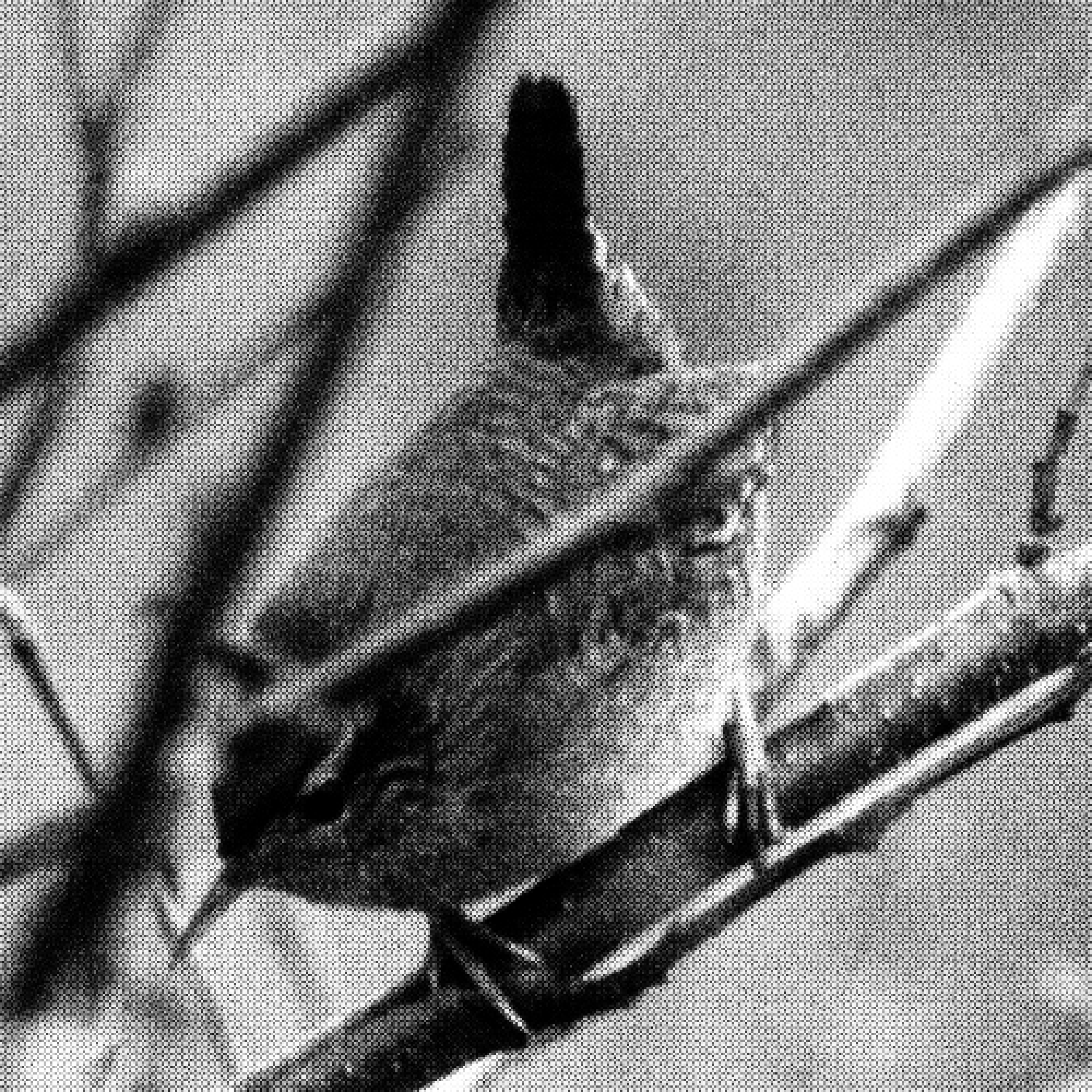Mosaic of a Wren.

This is actually the raw image content, all interpolation de-activated, scaled for better view. Obviously, there is a mosaic pattern in there.

And this is the sensor matrix. I had read about it, but never seen it. Did you ever notice it before? I did not. The reason is that mostly any image conversion will, as a very first step, de-mosaic the image. The mosaic comes from the need to get color information: a cmos is indifferent to wavelength, so we place colored “sunglasses” on every pixel. The mosaic shows the arrangement of different colors.

Using a Fujifilm X-T4 camera, my sensor is an “X-Trans” sensor. In consequence, there are 2x2 block patches of green surrounded by red-green-blue lines; there is some 3x3 symmetry on the overall pattern. Conventional Bayer sensors rather alternate color filters on the pixels (2x2 symmetry). More on that below.

Markesteijn Madness

People have of course tried to solve this. I noticed this first in RawTherapee, where one has control over the demosaic settings. Demosaicing seems to be an issue with Fuji sensors, and, pixel peeping at my photos in the stable version of RawTherapee, I would say it remains an unresolved one.

If I demosaic “Mono”, I get the raw mosaic - essentially no demosaicing, just conversion to grayscale.

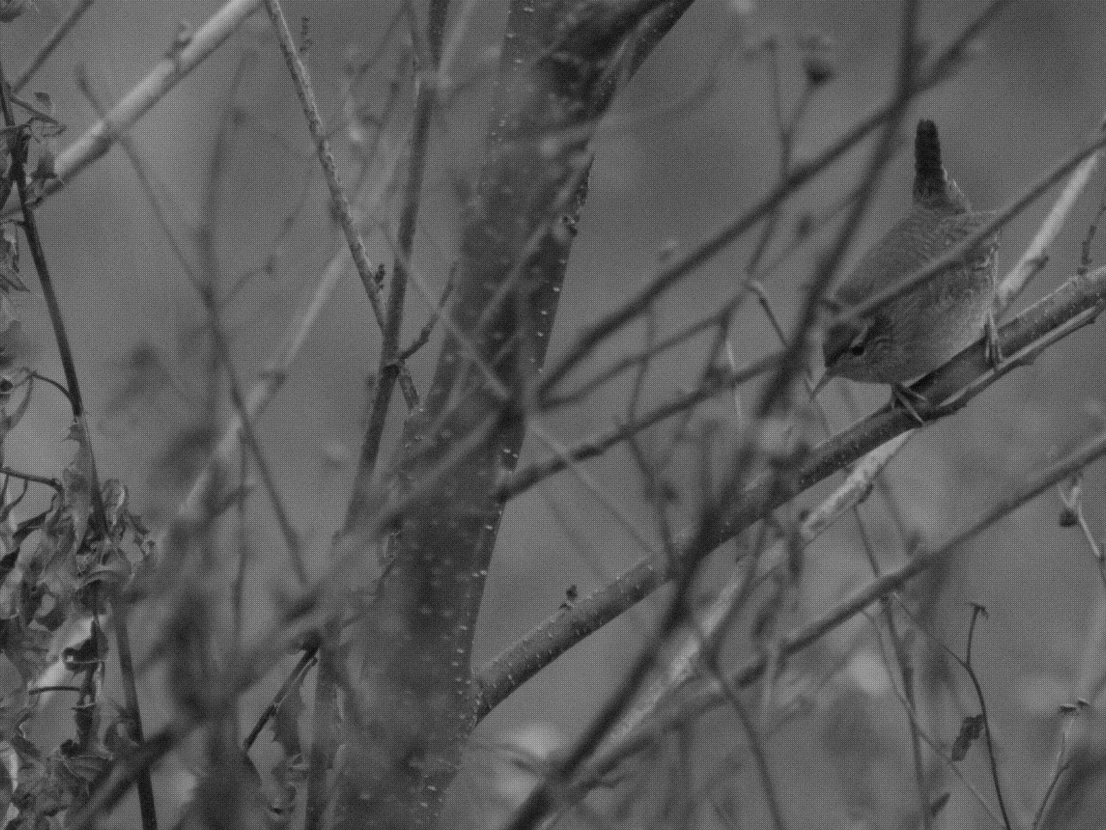Mosaic of a Wren. Again. But different software.

If I demosaic with the Markesteijn algorithm, I get better contrast, yet a lot of pixel noise, showing in a rugged histogram.

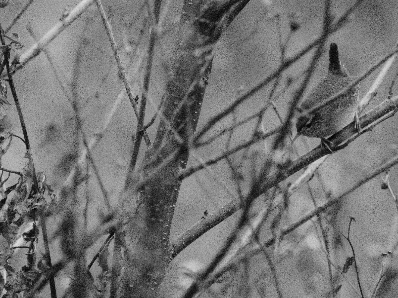The mosaic removed by Mr. Markesteijn in RawTherapee.

Despite the contrast issues, I find the first image sharper when looking at it from a certain distance that is just enough to let my eye interpolate the pixels, but not too far to suffer from my limited eyesight. Some noise and blur in the demosaiced one jump out. Also, some lookup tables (“film simulations”) just blow out the colors on some images, which I find looks similar to JPG compression artifacts. That is just an impression, calling for more investigate!

I had trouble finding a Markesteijn reference, except for the code above. There is a dead crosslink in that code. The actual C code is admittedly hard to comprehend for me as a spoiled python kid, yet there are comments in the file linked above, and from what I see those steps are accurately executed. The algorithm contains the following steps:

Map a green hexagon around each non-green pixel and vice versa
Set green1 and green3 to the minimum and maximum allowed values
Interpolate green horizontally, vertically, and along both diagonals
Recalculate green from interpolated values of closer pixels
Interpolate red and blue values for solitary green pixels
Interpolate red for blue pixels and vice versa
Fill in red and blue for 2x2 blocks of green
Convert to CIELab and differentiate in all directions
Build homogeneity maps from the derivatives
Average the most homogenous pixels for the final result

Critical here are averaging and interpolation: missing color values are filled with neighbours info.

Monochrome Sensors

I do have several tinkering cams lying around; an Odroid Cam and an ArduCam, as well as a noname amazon board with a Sony CMOS and an M12 mount. (Gear addiction at all levels - this article is for coping, after all.) One of the better ones has 12 Megapixels, monochrome (i.e. capturing light of any wavelength). This shall be our reference for a thought experiment.

My X-Trans IV, in comparison, has 26.1MP. But let us, for the sake of simplicity, imagine a 24MP sensor with Bayer filter layout. Each group of four pixels would have one Red, two Green, one Blue pixel. The green ones are spaced evenly on every second position. But that is just half of the pixels! Those essentially contribute all the green color information for the surrounding pixels. In other words, the ones in between are interpolated!

Sure, interpolation is more accurate than “no prior information”, and R, G and B might be associated through lightness. However, rigorously, from an information perspective, we have at maximum every second position covered.

This cripples an expensive 24MP Bayer sensor into a 12MP sensor, the level of a tinkering cam. In other words: the color information we get in modern sensors comes at a cost of resolution. Resolution, here, is to be understood in the correct way: resolution is the minimum distance of two points that could still be identified as separate. If each pixel were monochrome, we can have two light spot pixels separated by a dark pixel: resolution is exactly two pixel widths. In Bayer layout, these three would merge; one would get at best four pixel-to-pixel distances.

Back to the X-Trans layout: there is some controversy whether it can actually hold up to ist marketing claims. Given that there are more green pixels, and given a scene where green is relatively abundant and well correlated with overall luminosity, one could argue that the X-Trans would have the image information covered better (5/9 pixels of a well-represented color). Yet maybe that is just me rationalizing my investment in that system. In a reddish scene, Bayer has the advantage.

Color Science

Recovering colors is actually a fun venture which I have long neglected. There is white balance, there are film simulations. Yet those come in post processing. And post processing is just a new topic for me; I haven’t bothered by now. If I want to get rid of the Markesteijn artifacts, I usually have to apply two iterations of a 3x3 median filter. But that, in turn, is an effective reduction of resolution as well.

Most modern camera brands are quite good at covering up the partial missing information. Yet they do so by interpolating and blurring. What matters for the raw image are lens properties (ideally neutral) and the sensor.

Modern >40MP sensors might be the way to go, but often lenses cannot resolve that pixel density, or are expensive.

Conclusion

As demonstrated above, having color in images comes at a severe cost for resolution and sharpness. People probably learn that in photography school, while I was probably on a bathroom break.

I like sharp images, and this was a disappointing (but also exciting) discovery. Now, I am tempted to get a monochrome camera, and maybe some manufacturer will read this and manufacture one for me. But maybe that is just my gear trading addiction, again. I should rather write my own RBF demosaicing algorithm. …

A Custom Interpolator

This section was added on <2023-01-16 Mon>.

… and that is what I did!

Feel free to download the image here.

Interpolation/Demosaicing Code

Here you go.

First, read in the image.

### library imports, as above
import rawpy as RAW
import matplotlib.pyplot as PLT
import numpy as NP
import skimage.io as IO
import skimage.exposure as EXP
import skimage.util as UTIL
import scipy.interpolate as INTP
from tqdm import tqdm as tqdm

# specify an image
path = 'images/wren_raw.RAF'
with RAW.imread(path) as raw_image:
    # the x-trans IV delivers 12 bit images.
    rgb = raw_image.raw_image.astype(float).copy() / 2**12

    # the post processed image is used as a reference to bring exposure to meaningful values.
    raw = raw_image.postprocess().astype(float) / 2**8
    rgb = EXP.match_histograms(rgb, NP.mean(raw, axis = 2))

# PLT.matshow(rgb, origin = 'upper', cmap = 'gray')
# PLT.show()

# remove the fuji raw frame of darkness
rgb = rgb[2:, :6252]

# PLT.hist(rgb.ravel())
# PLT.show()

img_original = rgb.copy()
IO.imsave('wren_mono_original.png', UTIL.img_as_uint(img_original[1650:2150, 2700:3200]))

Then, we need to prepare the calculations below, by extracting our image dimensions. Interpolation of the whole image at once is RAM overkill. I therefore loop over patches of the image, considering a small frame that is cropped off for every patch to avoid margin effects.

## prepare the output image
shape = rgb.shape
img_out = NP.zeros((shape[0], shape[1], 3))

step = 18
assert step % 3 == 0
# Homework: try other steps

margin = 3
assert margin % 3 == 0

window = step-2*margin

start = [margin, margin]
# n_shifts = [50,50] # good for testing
n_shifts = [(shape[0]-2*margin)//window, (shape[1]-2*margin)//window] # full image

We then need a mask for each color! The pattern is clear, but I did not know where it begins. I checked that heuristically on my sensor readout, and started assembling the green mask, then the others.

### Masks
masks = {}

# # generate mask: green
# assuming that the first row is a grid row, i.e. one with equal RGB
mask = NP.ones((step, step), dtype = bool)
mask[1::3, 2::3] = False
mask[2::3, 2::3] = False
mask[0::3, 0::3] = False
mask[0::3, 1::3] = False
masks['g'] = mask

## generate BLUE mask
mask = NP.logical_not(masks['g'])
# turn OFF the reds
mask[0::6, 0::6] = False
mask[0::6, 4::6] = False
mask[1::6, 2::6] = False
mask[2::6, 5::6] = False
mask[3::6, 1::6] = False
mask[3::6, 3::6] = False
mask[4::6, 5::6] = False
mask[5::6, 2::6] = False
masks['r'] = mask

masks['b'] = NP.logical_not(NP.logical_or(masks['g'], masks['r']))

## mask check plot
# for channel, color in enumerate('rgb'):
#     PLT.matshow(masks[color])
#     PLT.suptitle(color)
#     PLT.show()
#

Then, the image patches are iterated, and an interpolation of choice happens. There is some flexibility in the algorithm - luckily, this is what we do this for, after all.

for upper in tqdm(NP.arange(0, n_shifts[0]*window, window)):
    # for left in tqdm(NP.arange(0, n_shifts*window, window), leave = False):
    for left in NP.arange(0, n_shifts[1]*window, window):

        upper_left = [start[0]+upper-margin, start[1]+left-margin]
        img_crop = rgb[upper_left[0]:upper_left[0]+step, upper_left[1]:upper_left[1]+step].copy()
        # print (upper_left, step, img_crop.shape)

        ### loop colors
        # color = 'r' # testing
        # channel = 0

        # for _ in [True]:
        for channel, color in enumerate('rgb'):

            positions = NP.stack(list(zip(*NP.where(masks[color]))), axis = 0)
            # print (img_crop.shape, masks[color].shape)
            values = [img_crop[pos[0], pos[1]] for pos in positions]

            ### (A) RBF interpolator
            # print ('#'*8, 'creating interpolator', '#'*8)
            # https://docs.scipy.org/doc/scipy/reference/generated/scipy.interpolate.Rbf.html
            interpolator = INTP.Rbf(positions[:, 0], positions[:, 1], values \
                            , function = 'multiquadric' \
                            , epsilon = 1. if color in ['g'] else 3. \
                            , smooth = 0 # is a MUST here: function will go through nodal points \
                            )  # radial basis function interpolator instance

            ## interpolation function timing:
            # 'multiquadric': 5:51 # crisper than linear
            # 'linear': 5:30
            # 'thin_plate': 6:30 # bit less blurry
            # 'gaussian': 6:27 # grainy with default epsilon


            # ### (B) CloughTocher Interpolator
            # # https://docs.scipy.org/doc/scipy/reference/generated/scipy.interpolate.CloughTocher2DInterpolator.html#scipy.interpolate.CloughTocher2DInterpolator
            # # took longer
            # interpolator = INTP.CloughTocher2DInterpolator(positions, values)


            ### interpolate!
            # # print ('#'*8, 'interpolation', '#'*8)
            new_positions = NP.stack(list(zip(*NP.where(~masks[color]))), axis = 0)
            new_values = interpolator(new_positions[:, 0], new_positions[:, 1])

            # print ('#'*8, 'visualization', '#'*8)
            img_intp = img_crop.copy()
            img_intp[~masks[color]] = new_values

            # store values
            img_out[start[0]+upper:start[0]+upper+window, start[1]+left:start[1]+left+window, channel] = img_intp[margin:margin+window, margin:margin+window]

Finally, save and plot the images for comparison, both monochrome and color.

# some cosmetics
img_out = img_out[start[0]:start[0]+n_shifts[0]*window, start[1]:start[1]+n_shifts[1]*window, :]
img_out[img_out > 1.] = 1.
img_out[img_out < 0.] = 0.

# cropping to the same size as above
img_out = img_out[1650:2150, 2700:3200]

## saving
IO.imsave('wren_rgb_rbf.png', ((img_out * 2**8)//1).astype(NP.uint8))
IO.imsave('wren_mono_rbf.png', ((img_out[:, :, 1] * 2**8)//1).astype(NP.uint8))

## plotting, side-by-side comparison
dpi = 300
fig = PLT.figure(dpi = dpi, figsize = (2*shape[0]/dpi,shape[1]/dpi))
fig.subplots_adjust(bottom=0, left=0, right=1, top=1, hspace = 0., wspace = 0.)

ax = fig.add_subplot(1,2,1)
img_cropped = rgb[start[0]:start[0]+n_shifts[0]*window, start[1]:start[1]+n_shifts[1]*window]
ax.matshow(img_cropped, cmap = 'gray')
ax.spines[:].set_visible(False)
ax.set_xticks([])
ax.set_yticks([])

ax = fig.add_subplot(1,2,2, sharex = ax, sharey = ax)
# ax.matshow(img_out, cmap = 'gray')
ax.imshow(img_out, origin = 'upper')
ax.spines[:].set_visible(False)
ax.set_xticks([])
ax.set_yticks([])

PLT.show()

This interpolation takes ~10 minutes on my machine; it is not practical, yet the result is honorable!

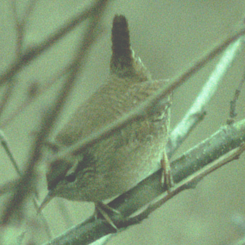
Troglodytes troglodytes, green of jealousy (and missing white balance). Custom interpolation.

I did compare this to what comes out of RawTherapee, and see some advantages. I like especially the monochrome green channel. But that could be due to the color of this particular image.

There remains a lot to explore!

Discussion

Some things are missing, compared to straight out-of-camera JPG, though:

White balance is off.
Contrast is low.
The noise remainder could be treated with some smoothing.
You might want to add a LUT (“film simulation”).

But maybe that can be done by storing a TIF and continue editing in RawTherapee!

Or, instead, there is actually a “better” demosaicing in RawTherapee directly, which is called “fast”, and discouraged in their Wiki. For my narrowly cropped wren, “fast” produced much fewer visible artifacts, and I found the overall image more appealing.

Yet ultimately, it would be much appreciated if Fuji revealed their algorithms: the in-camera post processing is quite astonishing and to the point!

Troglodytes troglodytes, the one and only: if you didn’t crop it, it was no wren. Fuji in-camera JPG conversion.

Summary

I hope you found this entertaining. Or informative. Or neither.

Have fun photographing, folks! Most photos herein were captured in the Antwerp Zoo.

Thank you for reading!

Photography: Megapixel Conspiracy

... and a Tamron SP 300mm f/2.8 review

Falk Mielke, University of Antwerp, January 10, 2023

Motivation

Table of Contents

Lens Review: Tamron SP 300mm f/2.8 LD IF

Introduction

Strengths

Limitations

The Good

The Bad

The Ugly

Sample Images

Summary

Demosaicing and the Megapixel Conspiracy

Mosaic Data

Markesteijn Madness

Monochrome Sensors

Color Science

Conclusion

A Custom Interpolator

Interpolation/Demosaicing Code

Discussion

Summary