(You can download this notebook here.)

Motivation

Recently, we suspected and confirmed an interesting relation of body part growth in piglets. This required dissecting cadavers and weighing several parts (such as head, thorax and hind part). Yet it turns out that I do not have too many piglets in my freezer (luckily) to get to statistically relevant sample sizes.

However, I do have a lot of piglet videos! Assuming that these animals are of rather homogeneous density, the segmented lateral projection of body surface should at least correlate with the segment masses. Hence, this should work like CT segmentation: take an image, color the body parts with a paint brush, and measure the colored area.

So far, so good… but i have A LOT OF piglet videos. Coloring all of them with a photoshop brush is just too laborious, even though rough is enough.

I have some image processing tricks up my sleeve to get this whole procedure semi-automated. Below you find it. A lot could be reported about the videos and the data, and I hope to do that soon in my thesis and in publication. Yet for now, for time constraints, I will just provide the code blocks and briefly explain what they do. In the end you find the whole tool for download. A lot of heuristics are in here, but because my data set is rather standardized, roll-out should be trivial.

I hope this procedure is of use to someone.

Table of Contents

1. Motivation
2. Moving Piglet Detection
3. Manual Segmentation: Draw Two Lines
4. Area Calculation
5. Summary

Moving Piglet Detection

Take a frame from a video of a moving piglet. The task is to find the animal and separate it from background. This is not trivial from the frame alone.

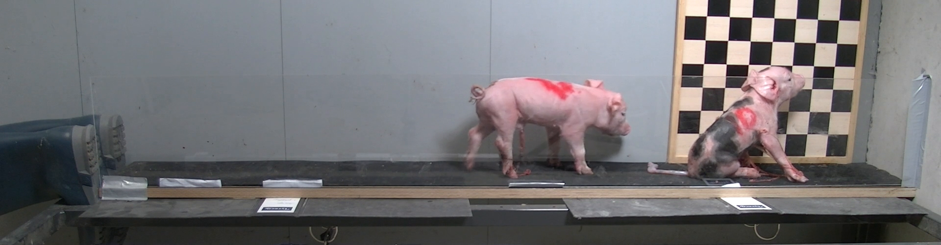
But those are videos, so let’s go a bit back in time! We can extract two frames: one early, one after the piglet has moved one or two strides. The first one could also be a “flat field”, i.e. a snapshot of the empty scene.

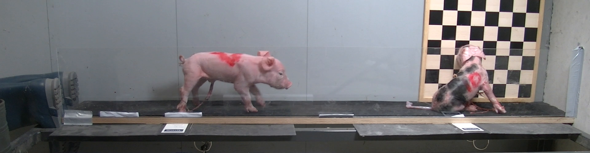
We can take the differential image, which is the (absolute of the) subtraction of the two images.

import os as OS
import numpy as NP
import scipy.ndimage as NDI
import matplotlib as MP
import matplotlib.pyplot as PLT
import skimage.util as SKU
import skimage.filters as SKF
import skimage.io as SKIO
MP.use('TkAgg')
dpi = 300

def FullDespine(ax):
    ax.spines[:].set_visible(False)
    ax.tick_params(bottom = False)
    ax.tick_params(left = False)
    ax.set_xticks([])
    ax.set_yticks([])

def PlotSingleImage(img, **kwargs):
    # plot a single image
    fig = PLT.figure(figsize = (float(img.shape[1])/dpi, float(img.shape[0])/dpi), dpi = 300)
    fig.subplots_adjust(bottom = 0, left = 0, top = 1, right = 1)
    ax = fig.add_subplot(1,1,1, aspect = 'equal')
    ax.imshow(img, **kwargs)
    FullDespine(ax)
    return fig



# load two images
reference_frame = 6100
test_frame = 6210

ref_img = PLT.imread(f'frames/{reference_frame:07.0f}.png').astype(float)
test_img = PLT.imread(f'frames/{test_frame:07.0f}.png').astype(float)

# calculate the differential image
diff_img = SKU.compare_images(ref_img, test_img, method = 'diff')

# plot the image
fig = PlotSingleImage(diff_img)

fig.savefig('./show/abs_diff.png', dpi = dpi)
PLT.close()

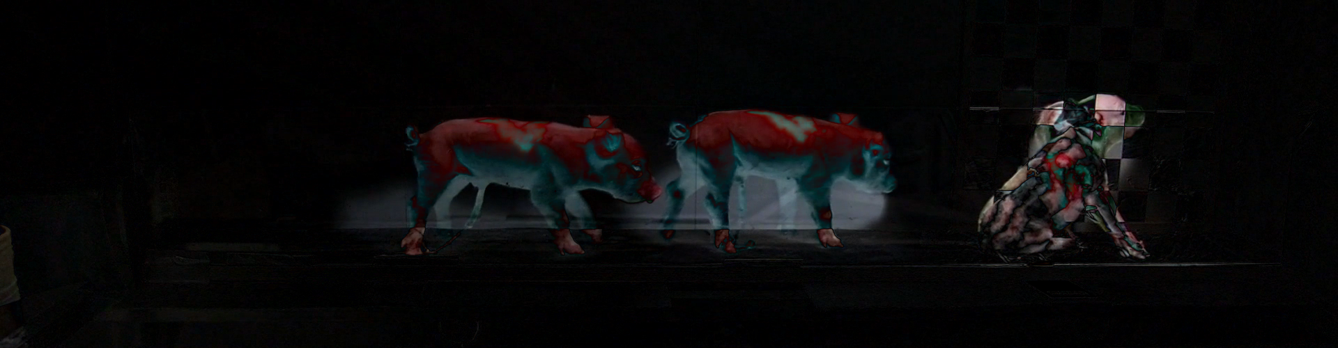
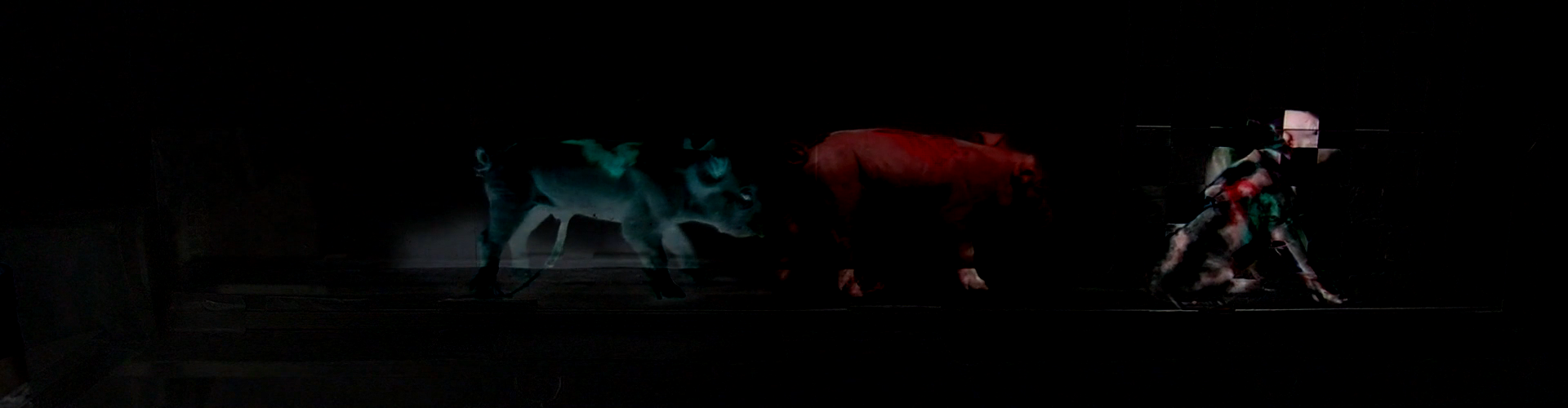
That’s even more psychodelic than the manual segmentation above! Yet there is hope: One can see where the focus animal left off, and where it arrived. And one can see the (stationary) movement of the other animal. The complexity arises from the RGB-Channels of the image and the absolute difference.

Take the plain difference, instead of the skimage function.

diff_channels = NP.subtract(test_img, ref_img)
fig = PlotSingleImage(diff_channels)
fig.savefig('./show/plain_diff.png', dpi = dpi)
PLT.close()

Clipping input data to the valid range for imshow with RGB data ([0..1] for floats or [0..255] for integers).

This is not too different from the previous attempt. However, notice that there moving piglet is green at takeoff, and red at landing. This has to do with the color channels: the diff is taken “per channel”, since the images in my case are actually a x by y by 3 numpy array. We are after the red piglet, so let’s look only at the red channel!

Another complication is that part of the runway lights up under the animal. This is the animals’ shadow cast onto it, which moves with the subject. Luckily, runway and shadow are grey (gray means: all color channels similarly), so the change affects all colors. Turns out that by subtracting the green from the red channel, I get the shadow largely removed. I’m so glad that piglets are pink!

Finally, the differential image is too sharp, and the extracted piglet shape might split into pieces (see below). This can be avoided by blurring just a bit.

# subtract green from red to remove shadow areas
diff_img = NP.subtract(diff_channels[:,:,0], diff_channels[:,:,1])

# only take positive difference
diff_img[diff_img < 0.] = 0.

# gaussian
diff_blur = NDI.gaussian_filter(diff_img, sigma = 5)

fig = PlotSingleImage(diff_blur, cmap = 'gray')
fig.savefig('./show/smooth_diff.png', dpi = dpi)
PLT.close()

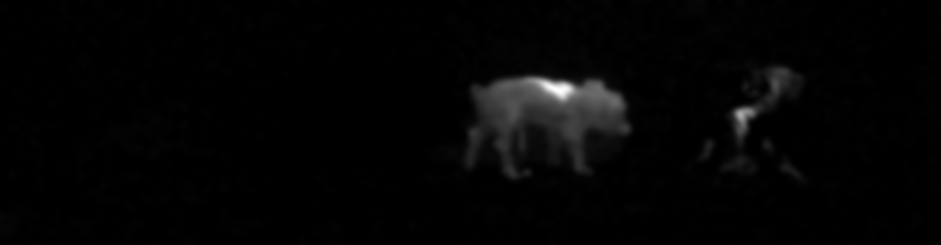
Looks much better! Next step is to identify (“label”) the light blocks with scipy.ndimage.label. Many more heuristics…

mask = diff_blur > 0.08
label_img, nb_labels = NDI.label(mask)
# print (label_img)

# find the biggest label
label_size = []
for lb in range(nb_labels):
    label_mask = label_img == lb + 1
    label_size.append(NP.sum(label_mask.ravel()))

# the biggest label is usually the animal which moved most.
biggen_label = NP.argmax(label_size) + 1
label_mask = label_img == biggen_label

fig = PlotSingleImage(label_mask, cmap = 'gray')
fig.savefig('./show/test_mask.png', dpi = dpi)
PLT.close()

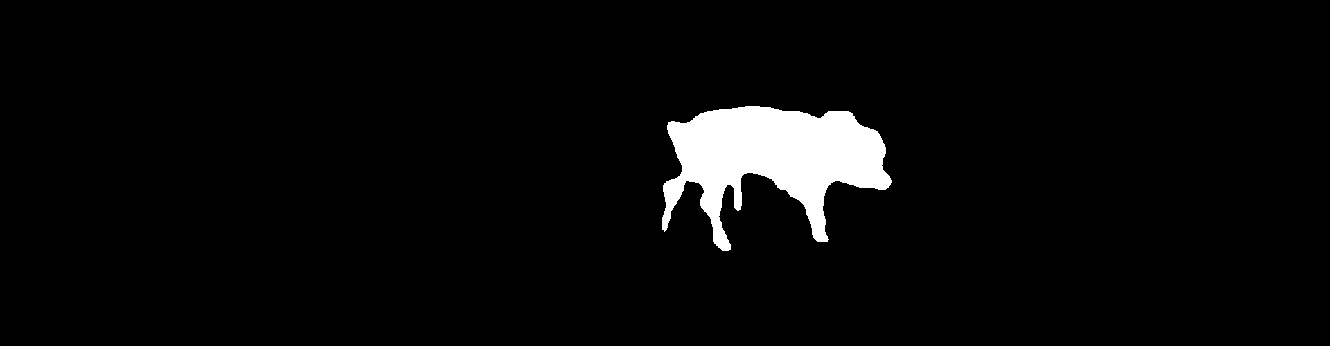
… And here we have it: a pretty accurate piglet mask!

Summary:

• take two frames
• subtract them (no absolute)
• look for channel-specific differences
• blur a bit
• label the light blobs

Manual Segmentation: Draw Two Lines

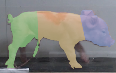
All right. I see the silhouette with the head, the thorax, hind part and limbs. If I see it, certainly a fancy deep learning AI could be programmed to see it as well…

… Or we just use a little GUI to draw two lines and store them. Who needs an AI anyways?

#!/usr/bin/env python3

# based on https://matplotlib.org/3.5.1/gallery/user_interfaces/embedding_in_tk_sgskip.html

import tkinter as TK

import matplotlib as MP
import matplotlib.pyplot as PLT
MP.use('TkAgg')

from matplotlib.backends.backend_tkagg import (
    FigureCanvasTkAgg, NavigationToolbar2Tk)
# Implement the default Matplotlib key bindings.
# from matplotlib.backend_bases import key_press_handler
from matplotlib.figure import Figure

import os as OS
import numpy as NP
import pandas as PD


image_files = ['test_mask.png']

for image_file in image_files:

    root = TK.Tk()
    root.wm_title("Embedding in Tk")

    fig = Figure(figsize=(5, 4), dpi=100)
    ax = fig.add_subplot(1, 1, 1, aspect = 'equal')

    img = PLT.imread(image_file)
    ax.imshow(img, cmap = 'gray', origin = 'upper')

    canvas = FigureCanvasTkAgg(fig, master=root)  # A tk.DrawingArea.
    canvas.draw()

    # pack_toolbar=False will make it easier to use a layout manager later on.
    toolbar = NavigationToolbar2Tk(canvas, root, pack_toolbar=False)
    toolbar.update()

    lines = {}
    line_handles = {}
    colors = { \
               'head': 'lightblue' \
               , 'hind': 'lightgreen' \
              }

    def DrawLines(label):
        # https://stackoverflow.com/questions/9136938/matplotlib-interactive-graphing-manually-drawing-lines-on-a-graph

        xy = NP.stack(fig.ginput(2), axis = 0)

        if line_handles.get(label, None) is not None:
            line_handles[label].remove()
        line_handles[label] = ax.plot(xy[:, 0], xy[:,1], color = colors[label])[0]


        canvas.draw()

        # print (label, '\n', xy)
        coords = PD.DataFrame(xy, columns = ['x', 'y'])
        lines[label] = coords

    def Save():
        out_file = f'{OS.path.splitext(image_file)[0]}.csv'
        df = PD.concat(lines, axis = 0)
        print (out_file)
        df.index.names = ['line','point']
        df.to_csv(out_file, sep = ';')

    def Quit():
        if len(lines) > 0:
            Save()
            print ('saved!')
        root.quit()



    def KeyHandler(event):
        if event.key == 'q':
            Quit()

        if event.key in ['h', '1']:
            DrawLines('head')
        if event.key in ['k', '2']:
            DrawLines('hind')

    # canvas.mpl_connect("key_press_event", lambda event: print(f"you pressed {event.key}"))
    canvas.mpl_connect("key_press_event", KeyHandler)

    button_lines = TK.Button(master=root, text="Lines", command=DrawLines)
    button_quit = TK.Button(master=root, text="Quit", command=Quit)

    # Packing order is important. Widgets are processed sequentially and if there
    # is no space left, because the window is too small, they are not displayed.
    # The canvas is rather flexible in its size, so we pack it last which makes
    # sure the UI controls are displayed as long as possible.
    button_quit.pack(side=TK.BOTTOM)
    button_lines.pack(side=TK.BOTTOM)
    toolbar.pack(side=TK.BOTTOM, fill=TK.X)
    canvas.get_tk_widget().pack(side=TK.TOP, fill=TK.BOTH, expand=1)

    TK.mainloop()

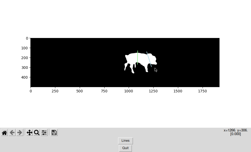
Sorry that this code is dirty and not fully commented, but for now, it works!

Area Calculation

Finally, based on the lines and the mask, the area can be calculated.

import os as OS
import numpy as NP
import pandas as PD

import matplotlib as MP
import matplotlib.pyplot as PLT
MP.use('TkAgg')

image_files = ['test_mask.png']

data = {}
for image_file in image_files:
    img = NP.array(PLT.imread(image_file), dtype = bool)
    # print (img.shape)

    line_file = OS.path.splitext(image_file)[0] + '.csv'
    lines = PD.read_csv(line_file, sep = ';', header = 0).set_index(['line', 'point'])
    # print (lines)

    mask_coords = NP.stack(NP.where(img), axis = 1)[:, [1,0]]
    total_area = mask_coords.shape[0]
    areas = {}
    for label in lines.index.levels[0].values:
        points = lines.loc[label, :].loc[[0, 1],['x', 'y']].values
        working_coords = mask_coords.copy()
        # print (points)

        working_coords = working_coords - points[0,:]

        vec1 = NP.append(NP.diff(points, axis = 0), 0)
        vec2 = NP.cross(vec1, NP.append(NP.diff(points, axis = 0), 1000))

        vec1 = vec1[:2] / NP.linalg.norm(vec1)
        vec2 = vec2[:2] / NP.linalg.norm(vec2)
        # print (vec1, vec2, NP.dot(vec1, vec2))
        basis = NP.stack([vec2, vec1], axis = 1)

        working_coords = NP.dot(working_coords, basis)
        # print (working_coords)

        # areas
        x = working_coords[:, 0]
        area1 = NP.sum(x >= 0)
        area2 = NP.sum(x < 0)

        # assuming the cut off areas are smaller
        areas[label] = NP.round(NP.min([area1, area2])/total_area, 2)

    data[image_file] = areas

data = PD.DataFrame.from_dict(data).T
print (data.to_markdown(tablefmt="orgtbl"))

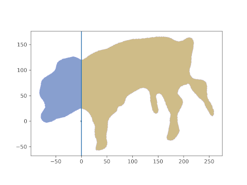
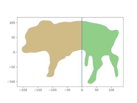
And, behold, this is the resulting area. The head is about 21%, the hind part about 39% of the lateral projection area. The middle part is what’s missing to 100%, i.e. about 40% in this case.

Note that this last part was automatic and simple. And it is generalizable: if you can get any segment on the animal which is “framed” by two lines, its pixel area can be calculated as the “mid” part above.

To summarize the third step, it requires:

• taking the mask, converting it to pixel coordinates
• creating basis vectors from the drawn lines
• center and rotate the coordinates
• count pixels

and, viola, you have the areas of you image segments!

Summary

The test outcome above is promising, and the result perfectly lies within the range of values we found by dissection. The challenge is getting thresholds for the differential images right in the first step above. But hold on… Can’t we summarize steps 1-3 in one GUI? Of course we can! You can download it here.

I am looking forward to roll out this procedure to a bigger data set, quickly extracting area measures from my animals.