(You can download this notebook here.)
Although I had hoped to avoid it, I recently dug into the world of automated video digitization. Namely, I trained a neural network with deeplabcut to give me lots of landmarks for my old piglet recordings. Those are hours of video, training was astonishingly succesful.
One immediate problem of such an amount of video is that you need to separate the relevant from the trash. (I intentionally formulated vaguely so that those of my readers with an affiliation to online movie streaming services will get hooked.) And because deep learning is “hip”, I anticipate that some futer colleagues might benefit from my attempts to solve the problem.
The goal is to take traces of multiple (limb) landmarks and atuomatically identify stride cycles, without having to manually annotate the video.
For those of you with less data (i.e. an amount that students could handle in reasonable time), I can highly recommend the ELAN video annotation software from colleagues at the MPI. I’ve used it for a long time, it has little to learn (but: keyboard shortcuts!) and is flexible and versatile, plus it is open source.
But now for the automatic part.
Table of Contents
Of course, I do this in my most familiar programming language, but you can easily port the procedure to others.
import numpy as NP # numeric operations
import pandas as PD # data storage and i/o
import scipy.signal as SIG # signal processing (mainly 1d)
import skimage as SKI # 2d signal processing
from skimage import feature as FEAT # "features" on 2d data

import matplotlib as MP # plotting
import matplotlib.pyplot as PLT

# useful shorthands
xy = ['x', 'y']
xyl = xy + ['likelihood']
dpi = 100
I will also reactivate my old friend Procrustes in this post (toolbox for download).
import SuperimpositionToolbox as ST
Example Data
This is what deeplabcut spit out after days of preparation, weeks of training and seconds of labeling:
You see on this short example that most of the time, nothing spectacular happens. Yet on a few occasions, the animal is moving, and there might be a full stride cycle. This is what we are trying to extract.
Here is the data:
framerate = 50 # frames per second
trace = PD.read_csv('cycles_example_trace.csv', sep = ';', header = [0,1]).set_index(('bodyparts','coords'))
trace.index = (trace.index.values - trace.index.values[0])/framerate
trace.index.name = 'time'
print(trace.T.iloc[:10, :6].round(3).to_markdown(index = True).replace(':|', '-+').replace('|:', '|-'))
|                         |     0.0 |    0.02 |    0.04 |    0.06 |    0.08 |     0.1 |
|-------------------------|---------+---------+---------+---------+---------+---------+
| ('snout', 'x')          | 615     | 607.514 | 600.908 | 596.479 | 591.301 | 587.299 |
| ('snout', 'y')          | 149.325 | 160.663 | 173.403 | 179.75  | 187.775 | 195.634 |
| ('snout', 'likelihood') |   1     |   0.999 |   1     |   1     |   1     |   1     |
| ('eye', 'x')            | 584.4   | 578.644 | 573.638 | 568.485 | 562.76  | 557.214 |
| ('eye', 'y')            | 111.137 | 121.162 | 130.867 | 139.213 | 145.05  | 153.298 |
| ('eye', 'likelihood')   |   1     |   1     |   1     |   1     |   1     |   1     |
| ('ear', 'x')            | 552.8   | 550.952 | 544.992 | 538.487 | 535.367 | 534.582 |
| ('ear', 'y')            |  85.473 |  94.946 | 101.946 | 112.196 | 117.147 | 125.438 |
| ('ear', 'likelihood')   |   0.997 |   0.97  |   0.998 |   1     |   1     |   0.738 |
| ('withers', 'x')        | 366.482 | 362.518 | 350.087 | 570.371 | 345.195 | 331.925 |
Usually I keep time in the rows (zero’th axis in numpy and pandas), but transpose improves the display. You can see that we have a time index, as well as (more than two) landmarks with \(x,y\)-coordinates and a likelihood. I will explain the likelihood below.
Shuffling Landmarks
Here is a complete list of landmarks:
landmarks = [ lm \
              for lm in NP.unique(trace.columns.get_level_values(0)) \
              ]
",".join(landmarks)
ankle,croup,ear,elbow,eye,fhoof,hhoof,hip,knee,metacarpal,metatarsal,scapula,shoulder,snout,tailbase,withers,wrist
For some of the calculations below (the Procrustes step), I will restrict the subset of landmarks to the limbs, and exclude those on the back and head.
exclude_landmarks = [  'snout', 'eye', 'ear' \
                       # , 'withers', 'croup', 'tailbase', 'scapula' \
                     ] # exclude head module and back
landmarks = [lm for lm in landmarks \
              if not (lm in exclude_landmarks) \
             ]
You mind find these landmark choices arbitrary. That is correct. But it is my data, so I may do what I like :) (evasion/lack of a good explanation tells you that this is the result of a tiresome trial-and-error procedure)
Finally, I will focus on the forelimb first.
limb = 'fl'
Hoof Speed
Fortunate for our analysis, the hoof landmarks move in a kind of regular pattern: during ground contact, their position is fixed, and in a swing, they move quickly.
Time for some audience participation: please
- get up now,
- walk across the room once, and
- observe the first derivative of your left foots position!
Meanwhile, I will store the labels of the three most distal landmarks.
hoof_landmarks = \
        {  'fl': ['wrist', 'metacarpal', 'fhoof'] \
         , 'hl': ['ankle', 'metatarsal', 'hhoof'] \
         }

# take coordinates of selected distal limb points
points = trace.loc[:, hoof_landmarks[limb]]
likelihoods = [ points.loc[:, (hlm, 'likelihood')].values.reshape((-1,1)) for hlm in hoof_landmarks[limb] ]
points = [ points.loc[:, [(hlm, coord) for coord in xy ]].values for hlm in hoof_landmarks[limb] ]
Images make the blog more interesting:
PLT.close()
fig = PLT.figure(figsize = (750/dpi, 250/dpi), dpi = dpi)
ax = fig.add_subplot(1,1,1, aspect = 'equal')
for i, pt in enumerate(points):
    ax.scatter(pt[:, 0], pt[:,1] \
               , s = 10 \
               , marker = 'o' \
               , alpha = 0.2+0.5*likelihoods[i] \
               , label = hoof_landmarks[limb][i]
               )

ax.legend(loc = 'best')
fname = 'images/hooflandmarks_time.png'
fig.savefig(fname, dpi = dpi)
fname
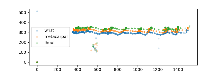
Behold the wavy patterns of hoof landmarks. Here is where you see the likelihood: because of the way I ser alpha above, they are visible as half-transparent points. The network is not always accurate (for example, it fails to digitize when my arm blocks view to the piglet on the video). However, probabilistic deep learning has the neat feature of telling you how sure it was of a given landmark at a given time. Low likelihood is a good criterium to discard data.
And more: we can use the likelihood to get a weighted average of landmarks.
# weighted averaging of distal limb points:
# sum up coordinates
point = NP.stack([pt * NP.dot(likh, NP.ones((1,2))) \
                  for likh, pt in zip(likelihoods, points)], axis = 2 \
                 )

# normalize by likelihood
normalizer = NP.dot( NP.sum( NP.concatenate(likelihoods, axis = 1), axis = 1).reshape((-1,1)) , NP.ones((1,2)) )
point = NP.divide(NP.sum(point, axis = 2), normalizer )
point[20:25, :]
| 483.85410117 | 342.20505423 | | 484.20987155 | 342.95532366 | | 485.42723442 | 345.55535856 | | 470.27070492 | 328.79654754 | | 465.69795559 | 325.10079237 |
Some smoothing might be justified. I only recently discovered theSavitsky-Golay Filter for this.
# smoothing
point = SIG.savgol_filter(point, window_length = 15, polyorder = 3, axis = 0)
point[20:25, :]
… quite drastic smoothing, but that is okay: this data is only used to extract time stamps, and I want to reduce the chance of false positives triggered by noise.
One more step: let’s take the first derivative, and we end up with a smoothed hoof speed.
# take the differential / spatial derivative
hoofspeed = NP.sum(NP.abs(NP.gradient(point, 5, axis = 0)), axis = 1)
Plotting that speed, you might see what you expected from the participation exercise above: peaks!

Quick note on the start and end: these are rather inaccurate periods, where the auto-detected landmarks are jumpy and have a low likelihood (I selected a bit extra on the sides), and where the smoothing above might produce artifacts.
The peaks above are the swing phases. They can vary in duration and height. Our next task will be the automatic selection of these repetitive peaks.
Cycles!
You can think of many ways of extracting the peak times. And many disciplines have solved varieties of similar problems. Some examples from the top of my head:
- Local maxima: Try to find the plain maxima. The problem is that they are not smooth, and there might be multiple peaks, and smoothing could alter the exact timing.
- Autocorrelation: Peaks are repetitive, so there would be a high auto correlation value at a characteristic time lag. However, the flat periods in between, and even some forms of signal noise, may contribute autocorrelation. One ends up with another variant of peak detection, and doesn’t come much closer to the goal.
- Wavelet Detection: This one comes from mass spectrometry, where there are particularly sharp peaks to be found in MS spectra. This is the strategy which worked for me.
A wavelet is a function of approximately the following form:
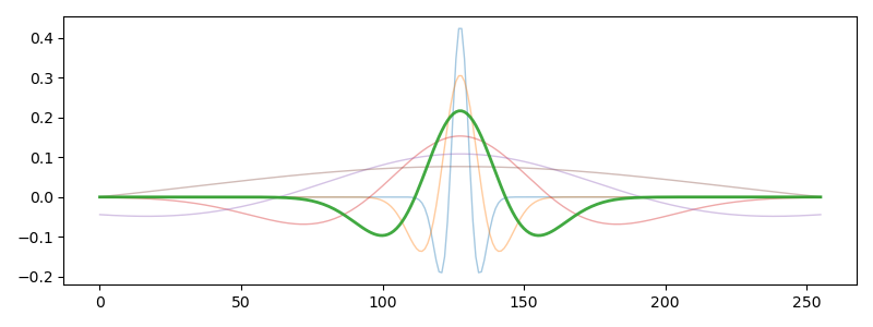
You see wavelets of different width. The emphasized green one is an intermediate width. Looks totally like a Mexican Hat, don’t you think?
Anyways. Here is the recipe for Continuous Wavelet Transform:
- generate a set of wavelets of varying width
- loop over the signal, along the time axis
- at every time point, for every wave width, calculate the correlation of the signal and the wavelet.
Or, in code: scipy.signal.cwt:
# wavelet transform with mexican head wavelets to find relative peaks
wv = 16
widths = NP.arange(1, wv)
# cwtmatrix = SIG.cwt(hoofspeed, SIG.ricker, widths)
cwtmatrix1 = SIG.cwt(hoofspeed, SIG.ricker, widths)
cwtmatrix2 = SIG.cwt(hoofspeed, SIG.morlet2, widths)
I am trying Ricker and Morlet here, because intuitively, a raw Morlet looks more like the peaks we are trying to detect. However, ricker works better:
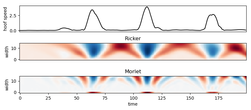
This is a solvable problem: The blue Ricker blobs are at the right time and have best match at approximately the width of the peaks we find. How can we find these blue blobs? Good news: the people from scikit image have done that before in skimage.featude.peak_local_max!
# find local maxima in the wavelet spectrogram
coords = FEAT.peak_local_max(cwtmatrix1.T, min_distance = 4, exclude_border = False)
time = coords[:, 0]
width = NP.array([widths[coord] for coord in coords[:, 1]])
Because this algorithm is sensitive to smaller blobs, we can filter based on some heuristics:
- cwt peaks should be above a threshold
- … and have a minimum peak width
threshold = 1.
sup = [idx for idx, t in enumerate(time) \
       if (hoofspeed[t] > threshold) \
       and (width[idx] > 2) \
       ] # the filter
time = time[sup]
width = width[sup]
peaks = NP.stack([time, width], axis = 1) # combine time/width
peaks = peaks[NP.argsort(peaks[:,0]), :] # sort by ascending time

peaks
| 9 | 15 | | 80 | 7 | | 183 | 7 | | 225 | 8 | | 275 | 9 | | 665 | 8 | | 712 | 8 | | 770 | 8 | | 811 | 8 | | 866 | 9 | | 910 | 3 | | 913 | 15 | | 923 | 4 |
Voilà!
See how most peaks have a characteristic width?
Quite good. But I still feel the urge to shift, stretch, and rotate!
Procrustes Optimization
Remember that we have more than just the hoof landmarks. Even though the hoof movement is repetitive, we should not disregard the rest of the information. We are looking for cyclical steady state locomotion. Here are the ones we can filter immediately:
- peaks are behind the end of the episode (shouldn’t happen; could be due to cutting)
- exclude too close peaks (i.e. too short/unsteady ground contacts or noise)
- too high inter-peak-interval (ipi)
- peaks overlap
- widths are too dissimilar
- think of more filters for your data!
def IsThisAGoodCycle(t1, w1, t2, w2):

    # first footfall after the end of the episode
    if t1 > trace.shape[0]:
        return False

    # second footfall after the end of the episode
    if t2 > trace.shape[0]:
        return False

    # peaks are way too far apart (my piglets don't move that slow)
    if t2-t1 > 120:
        return False

    # peaks overlap
    if t2-t1 < w1+w2:
        return False

    # too different widths = non-steady-state
    if w2-w1 > 6:
        return False

    # peak is good
    return True
We will loop peak pairs, i.e. compare one swing phase to the next.
# loop peak pairs
goodpeaks = []
for pk1, pk2 in zip(peaks[:-1, :], peaks[1:, :]):
    # reference timepoint
    t1, w1 = NP.sum(pk1), pk1[1]

    # comparison interval center
    t2, w2 = NP.sum(pk2), pk2[1]

    if not IsThisAGoodCycle(t1, w1, t2, w2):
        continue

    goodpeaks.append([t1, w1, t2, w2])

print(NP.stack(goodpeaks))
We’ve lost quite a few false positives. But we can do even better!
Here are some helper functions to quickly grab all landmarks at a certain time point.
NewConfiguration = lambda tp: NP.concatenate([ \
                     trace.iloc[[tp], :].loc[:, [(lm, coord) for coord in xyl]].values \
                     for lm in landmarks \
                     ], axis = 0)

config_store = {} # due to multiple grabs, it makes sense to store configs temporarily
def GetConfiguration(tp):
    configuration = config_store.get(tp, None)
    if configuration is not None:
        return configuration
    configuration = NewConfiguration(tp)
    config_store[tp] = configuration
    return configuration

MultiConfiguration = lambda tp: NP.concatenate([GetConfiguration(dtp) \
                                                for dtp in [tp-1, tp, tp, tp+1] \
                                                ], axis = 0)
landmarkcount_multiplier = 4

SupLikelihoods = lambda configuration: configuration[:, 2] > 0.9


# a function to quickly find a local minimum, given a start position
def FindLocalCenterMinimum(image, pos = None):
    if pos is None:
        pos = NP.array(image.shape) // 2
        print ('start:', pos)

    wl = 3 # window length
    window = image[pos[0]-wl:pos[0]+wl+1, pos[1]-wl:pos[1]+wl+1]

    if NP.all(NP.isnan(window)):
        # nan escape
        return pos

    # get local minimum
    d_pos = NP.unravel_index(NP.nanargmin(window), window.shape)

    if NP.sum(NP.abs(d_pos - wl*NP.ones((2,)))) == 0:
        # found minimum
        return pos

    # update position
    pos = pos + d_pos - wl

    if (pos[0] == 0) or (pos[0] + 1 == image.shape[0]) \
       or (pos[1] == 0) or (pos[1] + 1 == image.shape[1]):
        # escape border
        return None

    return FindLocalCenterMinimum(image, pos)
Steady state locomotion means that start and end of a cycle will have the animal in approximately the same configuration. This means, when we take landmarks at those timepoints, the Procrustes distance will be close to zero. It is hardly possible in reasonable time to cross compare all frames to find Procrustes Distance minima. Luckily, we have some clue where the cycle starts and ends! From the detected peaks, we roughly know the limb touch down (t + w) and can look in the proximity of that time point where the frame resemblance is best.
image_store = {}
PreWindow = lambda tx, wx: tx-wx//2
for t1, w1, t2, w2 in goodpeaks:
    # grab configurations
    # likelihoods can be very low (threshold!); min number of points above threshold; compare only those

    # store output as 2d image
    range_t1 = NP.arange(PreWindow(t1, w1), t1+w1+1)
    range_t2 = NP.arange(PreWindow(t2, w2), t2+w2+1)
    range_t2 = range_t2[range_t2 < trace.shape[0]]

    pd_image = NP.empty((len(range_t1), len(range_t2)))
    nl_image = NP.empty((len(range_t1), len(range_t2)))
    pd_image[:,:] = NP.nan
    nl_image[:,:] = NP.nan

    for i_ref, t_ref in enumerate(range_t1):
        # the reference configuration
        ref_configuration = MultiConfiguration(t_ref) # the configuration at the first peak
        ref_filter = SupLikelihoods(ref_configuration) # filter only well resolved landmarks
        ref_configuration[:, :2] = ST.Standardize(ref_configuration[:, :2])

        for i_candidate, t_candidate in enumerate(range_t2):

            # the candidate configuration
            candidate_configuration = MultiConfiguration(t_candidate) # comparison: configuration at second peak
            candidate_configuration[:, :2] = ST.Standardize(candidate_configuration[:, :2]) # filter only well resolved landmarks
            landmark_filter = NP.logical_and(ref_filter, SupLikelihoods(candidate_configuration))

            # minimum number of landmarks
            n_landmarks = NP.sum(landmark_filter)

            if n_landmarks < landmarkcount_multiplier*6:
                # too few landmarks
                continue

            # Procrustes!
            transformed, pd, _ = ST.Procrustes(  ref_configuration[landmark_filter, :2] \
                                               , candidate_configuration[landmark_filter, :2])
            pd_image[i_ref, i_candidate] = pd
            nl_image[i_ref, i_candidate] = n_landmarks

    if NP.sum(NP.logical_not(NP.isnan(pd_image))) < 6:
        # not enough comparisons found in the process
        continue
    image_store[t1] = { \
                          'tw': [t1, w1, t2, w2] \
                        , 'pd': pd_image \
                        , 'nl': nl_image \
                   }
We can plot the “image” of procrustes distances in the vicinity of the previously detected peak times:
t1 = goodpeaks[6][0]# 778
store = image_store[t1]
t1, w1, t2, w2 = store['tw']
pd_image = store['pd']

# find a local minimum
pos = FindLocalCenterMinimum(pd_image, pos = NP.array((w1//2, w2//2)))
print (pos)

PLT.close()
fig = PLT.figure(dpi = dpi)
fig.subplots_adjust(bottom = 0.1, left = 0.1, top = 0.99, right = 0.99, hspace = 0.05)
ax = PLT.subplot(1,1,1, aspect = 'equal')
ax.imshow(pd_image, origin = 'lower', cmap = 'RdBu')
ax.axvline(w2//2, color = 'w', lw = 0.5)
ax.axhline(w1//2, color = 'w', lw = 0.5)

# show minimum
if pos is not None:
    ax.axvline(pos[1]+0.1, color = 'y', lw = 0.5)
    ax.axhline(pos[0]+0.1, color = 'y', lw = 0.5)

ax.set_xticklabels(ax.get_xticks()-w2//2)
ax.set_yticklabels(ax.get_yticks()-w1//2)
ax.set_xlabel('start time offset')
ax.set_ylabel('end time offset')

fname = 'images/pd_image.png'
PLT.savefig(fname, dpi = dpi)
fname
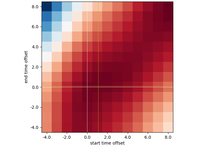
As we see, shifting the start and end times a bit (yellow cross) will give a better match of the landmark configurations in this example. The picture is not always that clear: there might be no minima at all, or the search for them might end up at the edges (indicating that our search space is too small). In my experience, the optimization procedure will usually be good for the good cycles.
Applying the procedure to all the cycles, but with the convenient skimage function to find the local minima:
cycles = []
for store in image_store.values():

    t1, w1, t2, w2 = store['tw']
    pd_image = store['pd']
    nl_image = store['nl']

    # again, we find the local image maxima to get the peaks.
    local_minima = FEAT.peak_local_max(-pd_image+NP.nanmax(pd_image) \
                                       , min_distance = 2 \
                                       , exclude_border = False \
                                       )

    if len(local_minima) == 0:
        # no local minimum was found
        continue

    # we will keep only that local minimum which is closest to the original peak position
    center_dist = NP.sum(NP.abs(local_minima - NP.array(pd_image.shape).reshape((1,-1))), axis = 1)
    best_idx = local_minima[NP.argmin(center_dist), :]

    pd_min = pd_image[best_idx[0],best_idx[1]]
    nl_min = nl_image[best_idx[0],best_idx[1]]


    # ... and that local minimum is our best guess for a cycle!
    cycles.append([PreWindow(t1, w1) + best_idx[0], PreWindow(t2, w2) + best_idx[1], NP.round(pd_min, 5), nl_min])

print (PD.DataFrame(cycles, columns = ['start', 'end', 'Procrustes distance', 'n landmarks']) \
                    .to_markdown(index = False) \
                    .replace(':|', '-+') \
       )
Seen from this table, Procrustes distance opens the door for another heuristic to filter “bad” cycles. Furthermore, you can check the stride distance, duration, and many other spatiotemporal parameters at this point to throw out garbage. But I’ll close here.
Summary
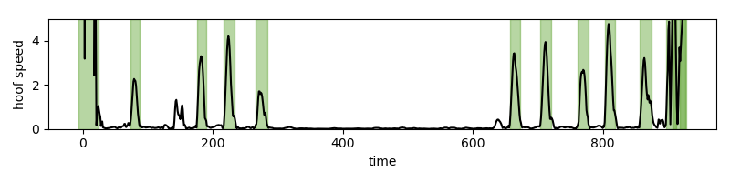
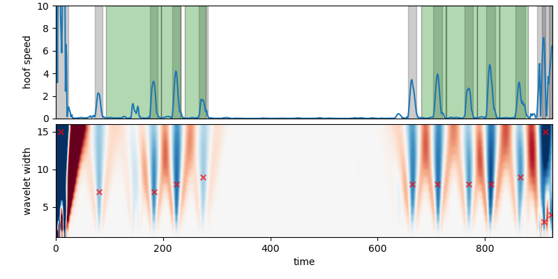
To re-iterate: Here is how you got a quite accurate estimate of cycle times.
- Use hoof speed, which has characteristic peaks in its temporal profile.
- Continuous Wavelet Transform can identify these peak times.
- Procrustes can compare configurations to refine cycle times.
- Along the way, use bespoke heuristics for your data set to filter out false positives.
PLT.close()
fig = PLT.figure(dpi = dpi, figsize = (800/dpi, 400/dpi))
fig.subplots_adjust(bottom = 0.15, left = 0.1, top = 0.98, right = 0.99, hspace = 0.05)
ax = PLT.subplot(2,1,1)
ax.plot(hoofspeed)
ax.set_xlim([0, len(hoofspeed)])
ax.set_ylim([0, 10])
ax.get_xaxis().set_visible(False)
for t, w in zip(time, width):
    ax.axvspan(t-w, t+w, color = 'k', alpha = 0.2)
for t1, t2, _, _ in cycles:
    ax.axvspan(t1, t2, facecolor = 'g', edgecolor = 'k', alpha = 0.3)

ax.set_ylabel('hoof speed')

ax = PLT.subplot(2,1,2, sharex = ax)
ax.imshow(cwtmatrix1, extent=[0, len(hoofspeed), 1, wv], cmap='RdBu', aspect='auto',
          vmax=abs(cwtmatrix1).max()*0.2, vmin=-abs(cwtmatrix1).max()*0.2, origin = 'lower')
ax.scatter(time, width, s = 30, color = 'r', marker = 'x', alpha = 0.7)
ax.set_xlabel('time')
ax.set_ylabel('wavelet width')

fname = 'images/timeline_overview.png'
PLT.savefig(fname, dpi = dpi)
fname
I would be happy to hear if this was useful for you, or if you maybe discovered improvements on one or the other intermediate step!
Thanks for reading!