This one is a technical post to document my method of calculating density distributions from CT scans. Because the data is huge, I cannot provide all of the image stacks on my webspace. However, do not hesitate to contact me.
The purpose of these notes is to take CT scan data and calculate (i) a density distribution based on the ct image gray values, (ii) calculate mass moment of inertia. The calculations are exerted on a controlled data set: the scan of a piglet femur and a couple of calibration objects.
import sys as SYS
import os as OS
import numpy as NP
import pandas as PD
import scipy.stats as STATS
import scipy.optimize as OPT

import matplotlib as MP
import matplotlib.pyplot as MPP

from skimage import io as SKIO

from tqdm import tqdm

MP.rc('text', usetex=True)
MP.rcParams['text.latex.preamble'] = r'\usepackage[cm]{sfmath}'
%pylab inline
Background
Imagine you have biological tissue in a CT scanner, and you would like to know the densities from the CT scan.
You might encounter several theoretical problems:
(1) X-ray sources have an emission spectrum, thus are not “monochromatic”.

from: Buzug, T. M., 2011. Computed tomography. In Springer handbook of medical technology (pp. 311-342). Springer, Berlin, Heidelberg. p.27 Fig 2.9.c
(2) Material has an absorbtion spectrum. Different chemical compounds will absorb different wavelengths differently.

from: Buzug, T. M., 2011. Computed tomography. In Springer handbook of medical technology (pp. 311-342). Springer, Berlin, Heidelberg. p.37 Fig 2.16
(3) Many kinds of artifacts distort the grey value scale.
Some of the problems above can be minimized; for example, metal filter plates can narrow the spectrum to high energy xray photons.
Still, there remain some challenges.
Experimental Setup
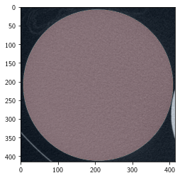
Herein I analyze CT scan taken on 10/03/2021 at the beautiful FlexCT Facility at my Universities campus.
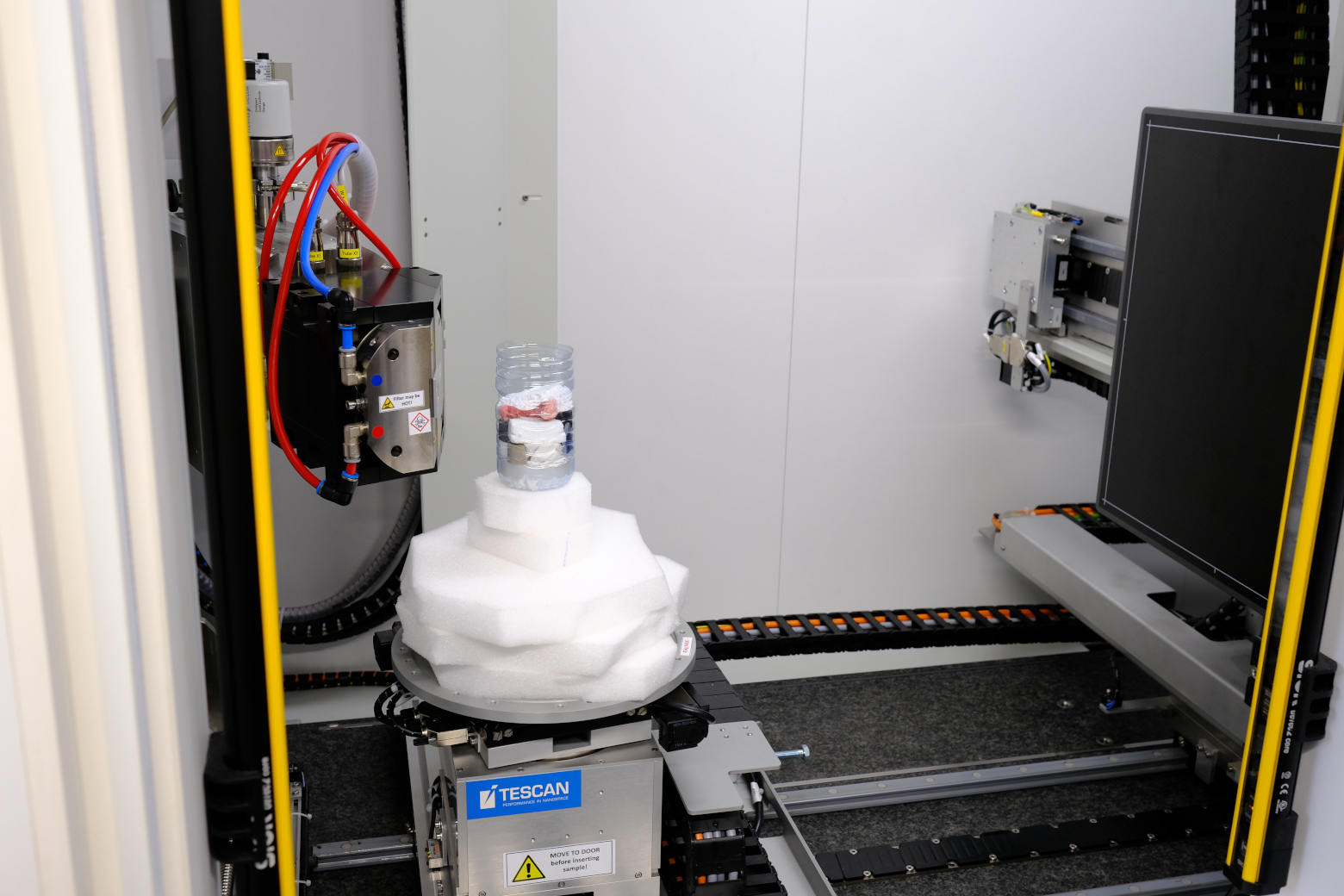
On the image, you see the scanner interior. The sample is contained in a plastic bottle. Most conspicuous is a piglet femur, pink, in the middle. It actually has metal markers glued to it. Below and beside this femur, there are several objects for density calibration:
- Diverse pieces of plastic; leftovers kindly provided by our mechanical workshop.
- Two Bruker Bone Mineral Density phantoms; hydroxiapatite cylinders with different calcium content, immersed in water. Thanks to Chris Broeckhoven for providing them!
You can also see white styrofoam pieces to hold everything in place.
Can we scan this? – Yes, we (s)can!
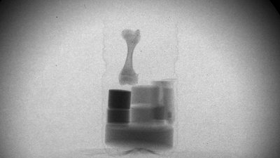
This gif shows the projections of the scan, which could be reconstructed to get a ct stack of 50 \(\mu m\) resolution.
Density Data
We know a couple of things about the items in that scan, which I compiled in the following table.
density_data = PD.read_csv('density_data.csv', sep = ';')
density_data['mean_grayvalue'] *= 1
density_data['measured_density'] *= 1
density_data
| material | reference_density | weight | volume | measured_density | mean_grayvalue | |
|---|---|---|---|---|---|---|
| 0 | air | 1.300000 | 8.257730e-08 | 6.352100e-08 | 1.300000 | 0.026784 |
| 1 | pp | 910.000000 | 7.779000e-03 | 8.490460e-06 | 916.204776 | 0.034165 |
| 2 | hmpe | 930.000000 | 4.602300e-02 | 4.943076e-05 | 931.059933 | 0.033877 |
| 3 | pe | 940.000000 | 8.103000e-03 | 8.527200e-06 | 950.253279 | 0.034210 |
| 4 | water | 999.800000 | 6.350830e-05 | 6.352000e-08 | 999.815740 | 0.035624 |
| 5 | pa6 | 1150.000000 | 1.313700e-02 | 1.135286e-05 | 1157.153632 | 0.035771 |
| 6 | pc | 1200.000000 | 1.768000e-03 | 1.511275e-06 | 1169.873314 | 0.035706 |
| 7 | pvc | 1300.000000 | 7.800000e-03 | 5.355602e-06 | 1456.418973 | 0.048084 |
| 8 | lowdens | 1254.090731 | 6.796600e-04 | 6.352012e-08 | 1254.090731 | 0.039906 |
| 9 | peek | 1320.000000 | 6.960000e-03 | 5.389127e-06 | 1291.489416 | 0.036409 |
| 10 | highdens | 1485.430465 | 9.787000e-05 | 6.588662e-08 | 1485.430465 | 0.047240 |
| 11 | ptfe | 2200.000000 | 8.724000e-03 | 3.949160e-06 | 2209.077373 | 0.043963 |
| 12 | femur | 1079.708657 | 5.271000e-03 | 4.881872e-06 | 1079.708657 | 0.037199 |
The columns: material is merely the label I gave to my specimens; reference_density is one taken from the literature (if available) or filled up with measured_density if there was no reference; measured_density is the measured density, calculated as quotient of weight (from a high accuracy scale) and volume (from \(50\mu m\) ct scan); mean_grayvalue is the arithmetic mean of all voxel values in the ct.
The code words lowdens and highdens are my labels for the hydroxyapatite phantoms (which reference a Bone Mineral density of \(0.25\) and \(0.75\) \(\frac{kg}{m^3}\), respectively). Note that I stick to SI units; different units will affect the outcome of the calculations below.
Let’s plot the theoretical (textbook) density against what I got by dividing weight (from a scale) by the volume (from CT):
dpi = 200
inch = 2.54
fig = MPP.figure(figsize = (12/inch, 12/inch), dpi = dpi)
ax = fig.add_subplot(1, 1, 1, aspect = 'equal')

ax.spines[['top', 'right']].set_visible(False)
ax.set_xlabel("reference density")
ax.set_ylabel("measured density")
ax.axline((0., 0), slope=1, color = '0.7', ls = '--', lw = 0.5)


for idx, measures in density_data.iterrows():


    material = measures['material']
    if material == 'femur':
        continue

    if any(PD.isnull(measures[['reference_density', 'measured_density']])):
        continue
    ax.scatter(measures['reference_density'], measures['measured_density'], s = 16\
               , marker = 'o', edgecolor = 'k', facecolor = 'none' )
    ax.text(measures['reference_density'], measures['measured_density']\
            , material.replace('_', ' '))

MPP.show()
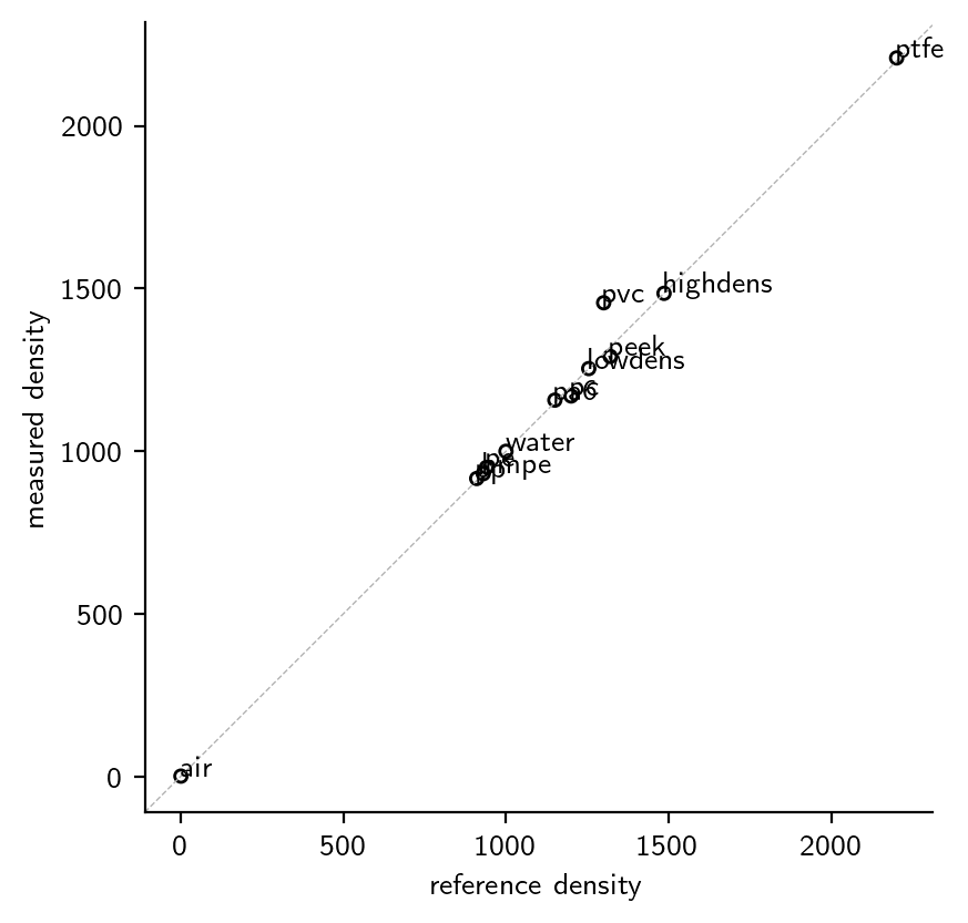
Most material densities approximately match textbook values.
The notable exception is the material labeled above as “PVC”. Generally, I only exclude outliers if there is a convincing proximate hypothesis to explain inconsistency with the data set. When I collected the material from the workshop, the colleague had initially missed PVC from the list. He then went to the workbench and brought me a gray, cylindrical piece, claiming it was PVC. From my measurements, I must assume it was not. Note that this hypothesis might be wrong, and PVC might have just been at some resonance with the chosen xray energy. However, it is not only the measured weight/volume ratio which is weird, but also the absorbtion (see below).
This justifies disregarding the supposed PVC data point.
Let us now look at the gray values.
fig = MPP.figure(figsize = (12/inch, 12/inch), dpi = dpi)
ax = fig.add_subplot(1, 1, 1)

ax.spines[['top', 'right']].set_visible(False)
ax.set_xlabel(r"measured density $\rho$")
ax.set_ylabel(r"mean gray value $\gamma$")

for idx, measures in density_data.iterrows():


    material = measures['material']
    if material in ['pvc', 'femur']: #
        continue

    if any(PD.isnull(measures[['reference_density', 'measured_density']])):
        continue


    ax.scatter(measures['measured_density'], measures['mean_grayvalue'] \
               , s = 16, marker = 'o', edgecolor = 'k', facecolor = 'none' )
    ax.text(measures['measured_density'], measures['mean_grayvalue'] \
            , material.replace('_', ' '))

MPP.show()

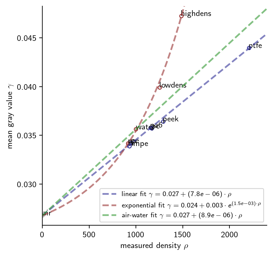
This plot is at the heart of my investigation: I would like to relate the gray values (\(y\)-axis) to physical density (\(x\)-axis).
Density Regression
To convert gray values to density, we need to estimate a conversion function. Such a function can be found by regression, given a reasonable hypothesis of how the values relate.
Here is a collection of functions that simplify different hypothesis fitting procedures.
## more general regression
def Regression(x, y, FitFunc = lambda x: x, init = NP.array([0]), verbose = False):
    '''Fits a linear fit of the form mx+b to the data'''

    # print ('regressing ', x, ' to ', y)

    Residual = lambda p, x, y, Fcn: NP.sum(NP.abs(NP.subtract(Fcn(p, x), y) )) #create error function for least squares fit

    #calculate best fitting parameters (i.e. m and b) using the error function
    out_params = OPT.minimize(Residual, init.copy(), args = (x, y, FitFunc), method = 'Nelder-Mead', tol = 1e-16)

    if verbose:
        print (out_params.success, out_params.x, out_params.nit)
    return out_params


RegressionCatalogue = {}

RegressionCatalogue['linear'] = { 'fcn': lambda params, x: params[0] + params[1]*x \
                                , 'inv': lambda params, x: (x - params[0])/ params[1] \
                                , 'init': NP.array((0.027, 0.01)) \
                                , 'label': lambda params: r'linear fit $\gamma = {:.3f} + ({:.1e}) \cdot \rho$'.format(*params) \
                                }

RegressionCatalogue['exponential'] = { 'fcn': lambda params, x: params[0] + params[1] *NP.exp(params[2] * x )  \
                                     , 'inv': lambda params, x: NP.log((x-params[0]) / params[1]) / params[2] \
                                     , 'init': NP.array((0.02, 0.007, 0.0009)) \
                                     , 'label': lambda params: r'exponential fit $\gamma = {:.3f} + {:.3f} \cdot e^{{ ({:.1e}) \cdot \rho}}$'.format(*params) \
                                    }
I can think of no single reasonable function that relates all points in the figure above.
However, what about splitting them into groups? One group are the synthetic polymers lying on a straight diagonal; the other group could be the materials which deviate upwards (i.e. show a higher than expected absorbtion).
group2 = ['air', 'pp', 'water', 'lowdens', 'highdens'] # team "exponential"
group1 = ['air'] + [material for material in density_data['material'].values \
         if (material not in group2 + ['femur', 'pvc'])] # team "linear"

colors = {material: (0.6, 0.2, 0.2) if material in group2 \
                      else (0.2, 0.2, 0.6) \
          for material in density_data['material'].values}
colors['air'] = (0.6, 0.6, 0.6) # air is in both groups

density_data['group1'] = [material in group1 for material in density_data['material'].values]
density_data['group2'] = [material in group2 for material in density_data['material'].values]
(1) Linear regression
First, fit the “linear” group of measurements. Results will be plotted below.
selection = 'linear'
linear_regression = RegressionCatalogue[selection]
linear_result = Regression(  \
                      x = density_data.loc[density_data['group1'].values, 'measured_density'].values \
                    , y = density_data.loc[density_data['group1'].values, 'mean_grayvalue'].values \
                    , FitFunc = linear_regression['fcn'] \
                    , init = linear_regression['init'] \
                    , verbose = True \
                    )
True [2.67743286e-02 7.77494528e-06] 185
(2) Exponential regression
And the same for the “exponential” group. It might be hard to get start values, because the observed value units are close to numeric accuracy, and because fitting an exponential (three degrees of freedom) through four points allows for some flexibility. So here is a little systematic start value search.
selection = 'exponential'
exponential_regression = RegressionCatalogue[selection]

x = density_data.loc[density_data['group2'].values, 'measured_density'].values
y = density_data.loc[density_data['group2'].values, 'mean_grayvalue'].values

good_results = []
a = 0.02
b = 0.007
for c in NP.linspace(0, 1.e-3, 101, endpoint = True):

    exponential_result = Regression(  \
              x = x \
            , y = y \
            , FitFunc = exponential_regression['fcn'] \
            , init = NP.array((a,b,c)) \
            , verbose = False \
            )
    if exponential_result.success and all(exponential_result.x >= 0):
        d = NP.sum(NP.abs(exponential_regression['fcn'](exponential_result.x, x) - y))
        good_results.append(NP.append(NP.array([a,b,c,d]), exponential_result.x))
        # print (good_results[-1])
good_results = NP.stack(good_results, axis = 0)
NP.median(good_results, axis = 0)
array([0.02      , 0.007     , 0.00072   , 0.00083707, 0.02418803,
       0.00259144, 0.00147133])
And here comes the actual regression:
selection = 'exponential'
exponential_regression = RegressionCatalogue[selection]

exponential_result = Regression(  \
                      x = density_data.loc[density_data['group2'].values, 'measured_density'].values \
                    , y = density_data.loc[density_data['group2'].values, 'mean_grayvalue'].values \
                    , FitFunc = exponential_regression['fcn'] \
                    , init = NP.array([0.02, 0.007, 0.0009]) #exponential_regression['init'] \
                    , verbose = True \
                    )
True [0.02418803 0.00259144 0.00147133] 262
Regression worked! But let’s look at another one:
(3) The Air-Water Axis
A third fit would be that connecting values for air and water. Might be reasonable, because most organic tissues have a high water content.
water_index = density_data.index.values[density_data.loc[:, 'material'].values == 'water'][0]
air_index = density_data.index.values[density_data.loc[:, 'material'].values == 'air'][0]
water_intercept = linear_result.x[0]
water_slope = (density_data.loc[water_index, 'mean_grayvalue'] - density_data.loc[air_index, 'mean_grayvalue']) \
            / (density_data.loc[water_index, 'measured_density'] - density_data.loc[air_index, 'measured_density'] \
              )
WaterFit = lambda x: water_intercept + water_slope * x
This is just another example. In fact, you can draw any line through the group of points - but we will check below which one gives plausible outcome. Even none-plausible outcomes are possible, for example:
(4) Constant Density
Thanks to Sam Van Wassenbergh for suggesting this. One can find a constant density value for all the segmented material. This would be a vertical line in the density-grayvalue plot. Regression makes no sense. But I will show this below when turning to the inertials.
Regression Comparison
Comparing all the regressions onto the data:
# plot function helpers
ρ = NP.linspace(0, 2400, 241, endpoint = True)

FIT = lambda catalogue, result: lambda x: catalogue['fcn'](result.x, x)
LinFcn = FIT(linear_regression, linear_result)
ExpFcn = FIT(exponential_regression, exponential_result)


# figure preparation
fig = MPP.figure(figsize = (12/inch, 12/inch), dpi = dpi)
ax = fig.add_subplot(1, 1, 1)

ax.spines[['top', 'right']].set_visible(False)
ax.set_xlabel(r"measured density $\rho$")
ax.set_ylabel(r"mean gray value $\gamma$")

# loop and plot materials
for idx, measures in density_data.iterrows():


    material = measures['material']
    if material in ['pvc', 'femur']: #
        continue

    if any(PD.isnull(measures[['reference_density', 'measured_density']])):
        continue


    ax.scatter(measures['measured_density'], measures['mean_grayvalue'] \
               , s = 16, marker = 'o', edgecolor = colors[material], facecolor = 'none' )
    ax.text(measures['measured_density'], measures['mean_grayvalue'] \
            , material.replace('_', ' '))

# plot regression outcomes
ylim = ax.get_ylim()

ax.plot(ρ, LinFcn(ρ) \
        , color = (0.2, 0.2, 0.6), ls = '--', lw = 2.0, alpha = 0.6 \
        , zorder = 10 \
        , label = linear_regression['label'](linear_result.x) \
       )
ax.plot(ρ, ExpFcn(ρ) \
        , color = (0.6, 0.2, 0.2), ls = '--', lw = 2.0, alpha = 0.6 \
        , zorder = 10 \
        , label = exponential_regression['label'](exponential_result.x) \
       )

ax.plot(ρ, WaterFit(ρ) \
        , color = (0.2, 0.6, 0.2), ls = '--', lw = 2.0, alpha = 0.6 \
        , zorder = 10 \
        , label = r'air-water fit $\gamma = {:.3f} + ({:.1e}) \cdot \rho$'.format(water_intercept, water_slope) \
       )

# cosmetics
ax.set_xlim([ρ[0], ρ[-1]])
ax.set_ylim(ylim)

ax.legend(loc = 4, fontsize = 8)

MPP.show()
The Femur Test, pt. 1
… and then along came the femur.
Of course, I have segmented it separating its fine outline from the rest. And I would like to know its density distribution (here) to calculate the center of mass and mass moment of Inertia (further below).
femur_grayvalues = NP.float64(NP.load('segments/v_femur.npy'))
print (femur_grayvalues.shape, femur_grayvalues.min(), femur_grayvalues.max())
(39054980,) 0.0 0.9999847412109375
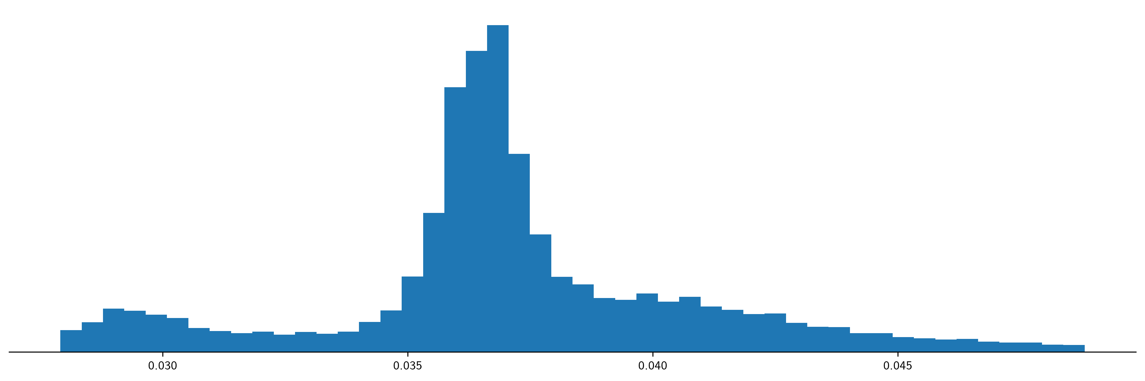
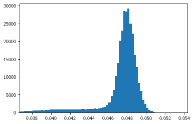
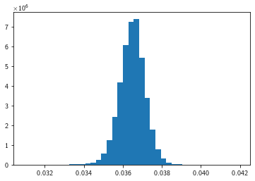
Let’s look at the gray value distribution:
f, ax = MPP.subplots(1,1, figsize = (16,5), dpi = 300)
value_range = NP.percentile(femur_grayvalues, [1,99])

ax.spines[['left', 'top', 'right']].set_visible(False)
ax.set_yticks([])
ax.hist(femur_grayvalues \
             , bins = NP.linspace(value_range[0], value_range[1], 49, endpoint = True) \
             , density = True);
We need some units and spatial parameters of the ct scan.
kg = 1; g = 1e-3 * kg
m3 = 1; cm3 = 1e-6 * m3
μm = 1e-6
voxel_edgelength = NP.float64(50 * μm)
voxelvolume_m3 = NP.float64(voxel_edgelength**3 * m3)
voxelvolume_m3
1.2499999999999997e-13
We also require the inverse regression function to convert from gray to density:
FIT = lambda catalogue, result: lambda x: catalogue['inv'](result, x)
LinInv = FIT(linear_regression, linear_result.x)
ExpInv = FIT(exponential_regression, exponential_result.x)
WaterInv = FIT(linear_regression, (water_intercept, water_slope))
Different conversions give different density distributions, and different calculated masses:
f, axes = MPP.subplots(1,3, figsize = (16,5), dpi = dpi)


for ax, Fcn, label in zip(axes, [LinInv, WaterInv, ExpInv], ['linear', 'water', 'exponential']):
    densities = Fcn(femur_grayvalues)
    densities = densities[~NP.isnan(densities)]
    value_range = NP.percentile(densities, [1,99])
    # densities = densities[(densities>=value_range[0]) & (densities<=value_range[1])]

    ax.hist(densities \
                 , bins = NP.linspace(value_range[0], value_range[1], 49, endpoint = True) \
                 , density = True \
           );
    ax.set_title(label)

    ax.spines[['left', 'top', 'right']].set_visible(False)
    ax.set_yticks([])

    weight = NP.sum(densities * voxelvolume_m3)
    print (label, weight)
    ax.set_xlabel(f"calculated weight: {weight/g:.3f} g")
linear 0.006545392030823989
water 0.005748516243244161


<ipython-input-5-1e248fed62a1>:27: RuntimeWarning: invalid value encountered in log
  , 'inv': lambda params, x: NP.log((x-params[0]) / params[1]) / params[2] \


exponential 0.005130278978770783
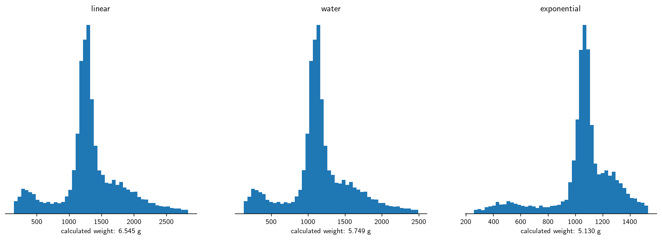
The true femur weight was determined to be 5.271g (including the beads).
ALL of the regressions presented here are wrong. The masses from linear regressions are too high, whereas the exponential fit gives too low voxel densities and mass.
Image Differentials
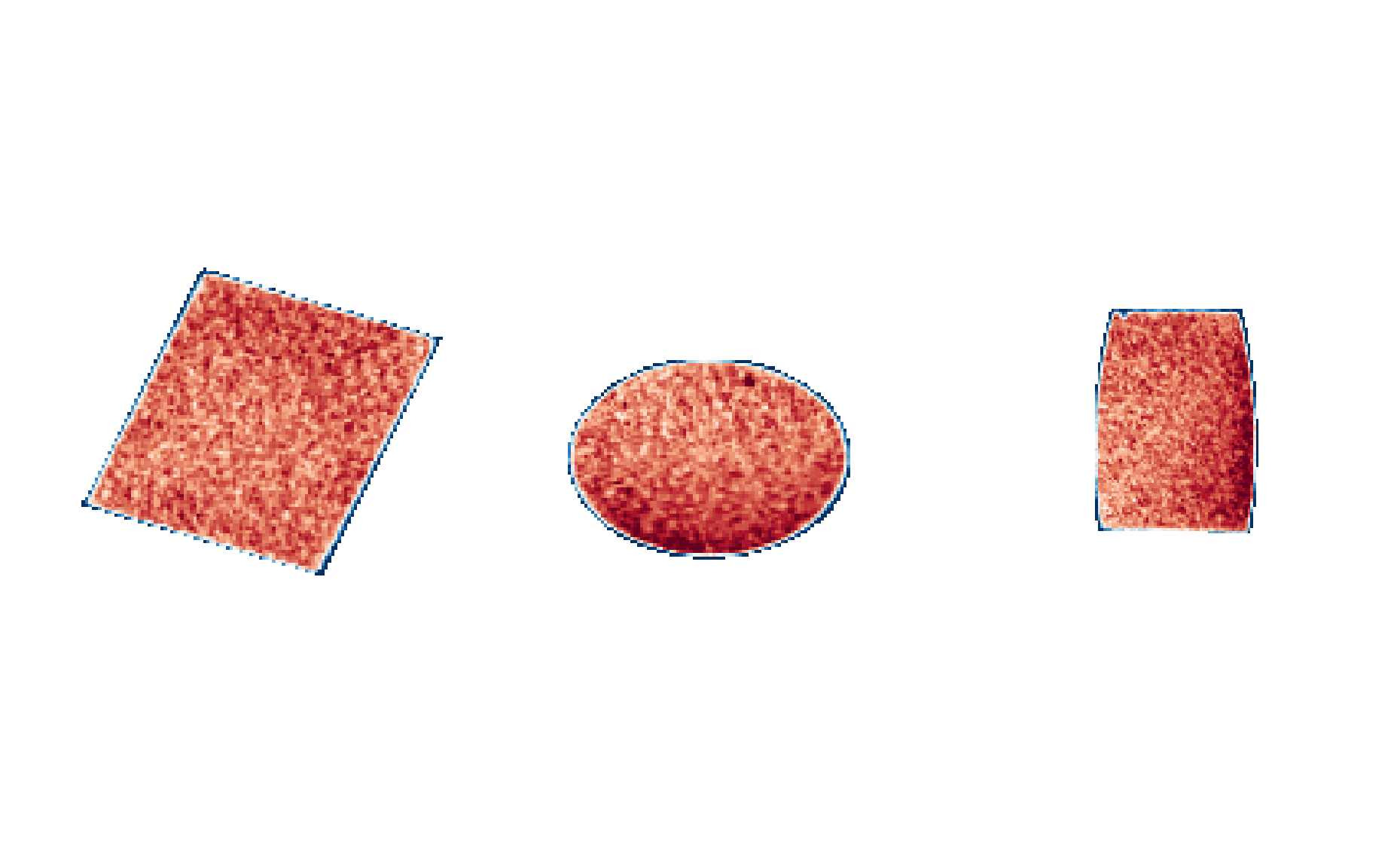
Let’s see where the regression conversion is off. Grab three test images from our data stack:
import tifffile as TIF
stack = TIF.imread('segments/d_ff_scan1.tiff')
stack.shape
(1791, 1512, 1512)
vmin, vmax = NP.percentile(femur_grayvalues, [1,99])
bits = 16
test_images = [stack[:,680,:], stack[1010,:,:], stack[350,:,:]]
test_images = list(map(lambda img: NP.array(img, dtype = NP.float64)/ 2**bits, test_images))
print ([(NP.min(img), NP.max(img)) for img in test_images])
[(0.0, 0.9999847412109375), (0.02362060546875, 0.05072021484375), (0.00128173828125, 0.9999847412109375)]
And see which images I arbitrarily selected:
fig, axes = MPP.subplots(2,len(test_images), gridspec_kw = dict(height_ratios = [0.9, 0.1]), dpi = 300)
fig.subplots_adjust(0., 0., 1., 1., 0.01, 0.01)


for ax, histax, img in zip(axes[0, :], axes[1, :], test_images):
    ax.spines[['left', 'top', 'right', 'bottom']].set_visible(False)
    ax.set_aspect('equal')
    ax.set_xticks([]), ax.set_yticks([])
    ax.imshow(img, cmap = 'gray', norm = None, vmin = vmin, vmax = vmax )


    histax.spines[['left', 'top', 'right']].set_visible(False)
    histax.set_yticks([])
    histax.hist(img.ravel() \
             , bins = NP.linspace(vmin, vmax, 49, endpoint = True) \
             , density = True \
       )
MPP.show();
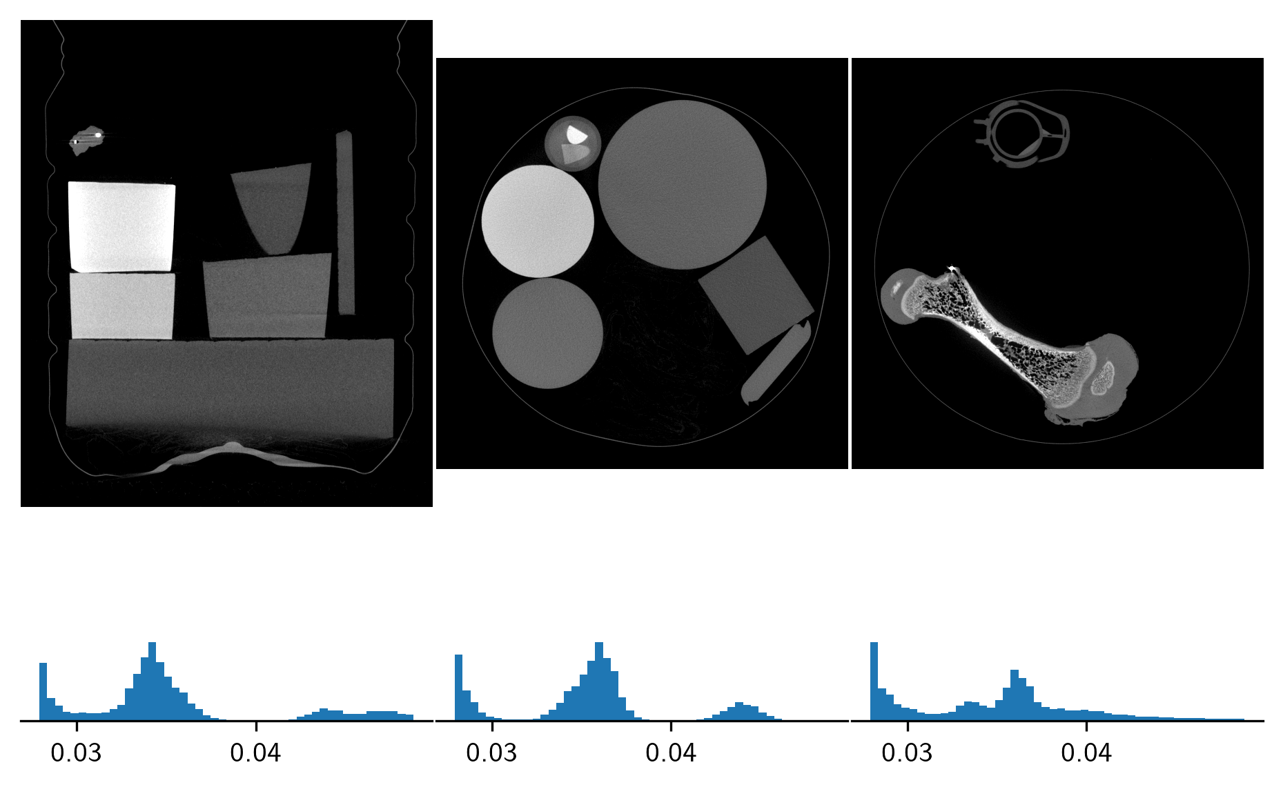
(histograms are the gray value distributions)
Convert them to density maps with the different regression functions:
labels = ['linear', 'water', 'exponential']
test_conversion = {label: {} for label in labels }
def NANtoZero(img):
    img[NP.isnan(img)] = 0.
    return img


for Fcn, label in zip([LinInv, WaterInv, ExpInv], labels):
    for idx, img in enumerate(test_images):
        test_conversion[label][idx] = NANtoZero(Fcn(img))
<ipython-input-5-1e248fed62a1>:27: RuntimeWarning: invalid value encountered in log
  , 'inv': lambda params, x: NP.log((x-params[0]) / params[1]) / params[2] \
# get limits
values = NP.concatenate([ \
          NP.subtract(test_conversion['exponential'][idx], test_conversion['linear'][idx]).ravel() \
          for idx in range(3)])
mean = NP.mean(values)
# values -= mean
vmin, vmax = NP.percentile(values, [1,99])
With this, we can map where the differences between linear and exponential are most prominent in our specimens:
fig, axes = MPP.subplots(2,len(test_images), gridspec_kw = dict(height_ratios = [0.9, 0.1]), dpi = 300)
fig.subplots_adjust(0., 0., 1., 1., 0.01, 0.01)


for ax, histax, idx in zip(axes[0, :], axes[1, :], range(3)):
    ax.spines[['left', 'top', 'right', 'bottom']].set_visible(False)
    ax.set_aspect('equal')
    ax.set_xticks([]), ax.set_yticks([])
    diffimg = NP.subtract(test_conversion['exponential'][idx], test_conversion['linear'][idx])

    ax.imshow(diffimg, cmap = 'RdBu', norm = None, vmin = vmin, vmax = vmax)


    histax.spines[['left', 'top', 'right']].set_visible(False)
    histax.set_yticks([])
    histax.hist(diffimg.ravel() \
             , bins = NP.linspace(vmin, vmax, 49, endpoint = True) \
             , density = True \
       )
MPP.show();
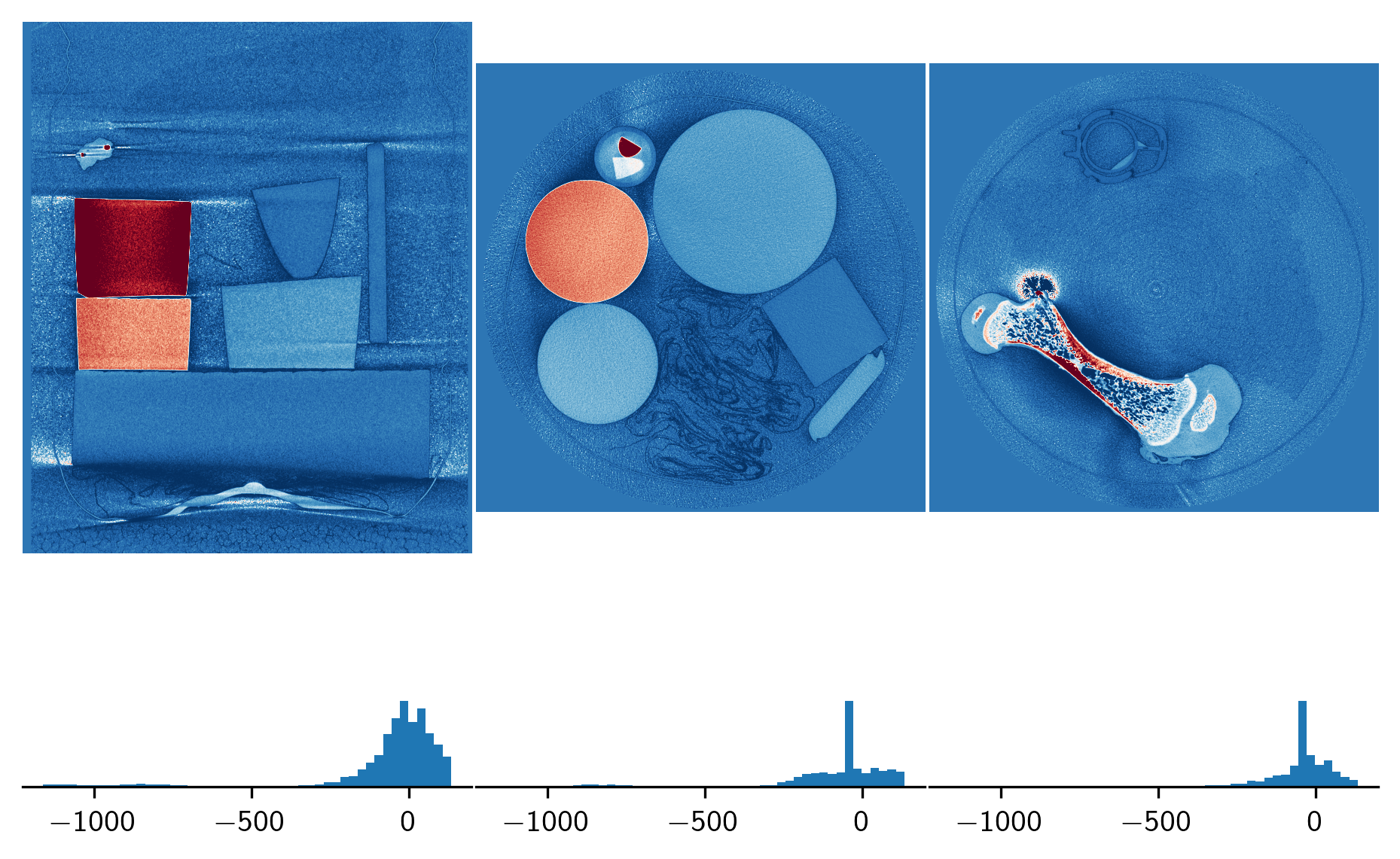
Interpretation:
The linear fit is considered the baseline.
Taking the exponential fit instead will reduce inferred density of high density areas (indicated by red color above). Consequently, the exponential fit underestimates the weight of the femur, as we saw above.
Conversely, low density areas get excess weight in the exponential fit.
Note that the image heatmaps are exaggerated by setting the color scale to percentile values. The actual difference seems to be small. However, these heatmaps show some rather subtle patterns which are either real (imperfect specimens), or artifacts of ct scans. See for example the concentric density variation within a cylinder (left image, dark red object) or a similar gradient concentric with the ct rotation (middle image). Also, there are quite extreme artifacts around the high density metal beads (right image).
True densities might even be better approximated by scaling the converted values ex post so that calculated weights match a known total weight, which I will apply below.
A brief recap:
- There are some materials which absorb more than expected. None of the materials I tested lie clearly below the linear reference line (which would indicate they are extra translucent to x-ray photons).
- The calculated density distribution (trivially) depends on which regression is used.
- Typical ct reconstruction effects become visible in all objects (circular artifacts in the heatmaps), but I did not quantify.
- A consequence is that none of the calculated density maps are perfect. Although none of them is homogeneous in gray values, it is reasonable to assume that the polymer specimens used herein were close to ideal and serve as a baseline.
- An exponential fit returns lower densities for each gray value than the linear fit (expected - the inverse of an exponential is a logarithmic curve). In consequence, the exponential regression usually underestimates the voxel densities.
Mass Moment of Inertia
What consequences does this inaccuracy have for mass moment of inertia? We’ll find out by calculating \(I\) for a couple of objects.
Here are the required formulas:
### I copied these functions from here:
# https://github.com/espressomd/espresso
# https://github.com/espressomd/espresso/blob/python/src/python/espressomd/rotation.py

def InertiaTensor(positions, masses):
    """
    Calculate the inertia tensor for given point masses
    at given positions.
    Parameters
    ----------
    positions : (N,3) array_like of :obj:`float`
        Point masses' positions.
    masses : (N,) array_like of :obj:`float`
    Returns
    -------
    (3,3) array_like of :obj:`float`
        Moment of inertia tensor.
    Notes
    -----
    See wikipedia_.
    .. _wikipedia: https://en.wikipedia.org/wiki/Moment_of_inertia#Inertia_tensor

    https://github.com/espressomd/espresso
    """
    inertia_tensor = NP.zeros((3, 3))
    for idx, pos in tqdm(enumerate(positions)):
        inertia_tensor += masses[idx] \
                        * ( NP.dot(pos, pos) * NP.identity(3) \
                            - NP.outer(pos, pos) \
                          )
    return inertia_tensor


CenterOfMass = lambda positions, masses: \
                    NP.average(positions, axis = 0, weights = masses)


def EigenAnalyze(squarematrix):
    # https://github.com/espressomd/espresso
    eigenvalues, eigenvectors = NP.linalg.eig(squarematrix)
    eigenvectors = NP.transpose(eigenvectors)

    # check for right-handedness
    if not NP.allclose(NP.cross(eigenvectors[0], eigenvectors[1]), eigenvectors[2]):
        eigenvectors[[0, 1], :] = eigenvectors[[1, 0], :]

    return eigenvalues, [eigenvectors[i, :] for i in range (eigenvectors.shape[0])]


def DiagonalizedInertiaTensor(positions, masses):
    """
    Calculate the diagonalized inertia tensor
    with respect to the center of mass
    for given point masses at given positions.
    Parameters
    ----------
    positions : (N,3) array_like of :obj:`float`
        Positions of the masses.
    masses : (N,) array_like of :obj:`float`
    Returns
    -------
    (3,) array_like of :obj:`float`
        Principal moments of inertia.
    (3,3) array_like of :obj:`float`
        Principal axes of inertia.
        Note that the second axis is the coordinate axis (same as input).

    https://github.com/espressomd/espresso
    """
    assert NP.array(masses).shape[0] == NP.array(positions).shape[0]

    positions = positions.copy() \
                    - CenterOfMass(positions, masses)
    inertia = InertiaTensor(positions, masses)
    eigenvalues, eigenvectors = EigenAnalyze(inertia)

    return inertia, eigenvalues, eigenvectors
Test 1: Synthetic Data
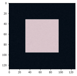
Good to start with an artificial data set (cube) with known outcome. This can exclude most of the errors in the functions above.
## arbitrary units
mass_unit = 1e-3 # 1 gram per unit
noise_unit = mass_unit/100 # 1% noise
space_unit = 1e-3 # 1mm
cube_mask = NP.zeros((128,128,128), dtype = bool)
cube_mask[32:96, 32:96, 32:96] = True
noise = NP.random.normal(0, noise_unit, cube_mask.shape)

cube = NP.array(cube_mask, dtype = NP.float64)
cube *= mass_unit
cube += noise

MPP.imshow(cube[:, cube.shape[1]//2, :], cmap = 'gray');
MPP.imshow(cube_mask[:, cube_mask.shape[1]//2, :], cmap = 'RdBu_r', alpha = 0.2);
MPP.gca().set_aspect('equal');
The Inertial calculation requires arrays of the voxel positions and masses.
# positions and grays
positions = NP.stack(NP.where(cube_mask)).T
masses = NP.array([cube[pos[0], pos[1], pos[2]] for pos in positions])

positions = NP.array(positions, dtype = NP.float64) * space_unit
print (positions.shape, masses.shape)
(262144, 3) (262144,)
With this, just call the function.
# Inertia calculation
_, I_calculated, _ = DiagonalizedInertiaTensor(positions, masses)
I_calculated
262144it [00:04, 52815.75it/s]


array([0.17891462, 0.17891977, 0.17891792])
Compare these to the theoretical result:
1/6 * NP.sum(cube) * ((96-32)*space_unit)**2
0.17896779222438164
The calculation seems to work as expected!
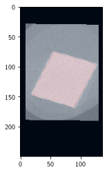
Test 2: A BMDensity Calibration Cylinder
I’ll also check one of the small hydroxyapatite cylinders, called “density phantoms”. The high density one deviates most from the linear regression, so errors should be emphasized.
# load the data
phantom = NP.array(TIF.imread('segments/d_highdens_cylinder.tiff'), dtype = NP.float64) / 2**bits
mask = NP.array(TIF.imread('segments/b_highdens_test.tiff') > 0, dtype = 'bool')

# and plot it
MPP.imshow(phantom[phantom.shape[0]//2, :, :], cmap = 'gray');
MPP.imshow(mask[mask.shape[0]//2, :, :], cmap = 'RdBu_r', alpha = 0.2);
MPP.gca().set_aspect('equal');
The true \(I\) of the cylinder can be calculated.
r = 2018.68*µm
h = 5096.21*µm
m = 0.09787*g
r,h,m
(0.00201868, 0.0050962099999999995, 9.787e-05)
I_zz = (1/2) * m*(r**2)
I_xx = I_yy = (1/12)*m*(3*(r**2)+(h**2))
I_xx, I_yy, I_zz
(3.1152480329437754e-10, 3.1152480329437754e-10, 1.9941349869634404e-10)
This should better also be the result of the numeric calculation. Let’s see!
As above, we need position and mass arrays.
# positions and grays
positions = NP.stack(NP.where(mask)).T
grays = NP.array([phantom[pos[0], pos[1], pos[2]] for pos in positions])

positions = NP.array(positions, dtype = NP.float64) * voxel_edgelength
print (positions.shape, grays.shape)
(302449, 3) (302449,)
Note that the distribution of gray values is rather wide, non-haussian, and has a “long tail” on the left:
MPP.hist(grays, bins = 100);
MPP.gca().set_xlim(NP.percentile(grays, [5,95]) + [-0.005, 0.005]);
NP.diff(NP.percentile(grays, [10,90]))
array([0.0038147])
Let’s look at the spatial distribution of this.
# and plot it
# vmin, vmax = NP.percentile(grays, [5,95])
vmin, vmax = [0.04, 0.05]
phantom2 = phantom.copy()
phantom2[NP.where(~mask)] = NP.nan

fig, axes = MPP.subplots(1,3, dpi = 300)
fig.subplots_adjust(0., 0., 1., 1., 0.01, 0.01)

axes[0].imshow(phantom2[phantom2.shape[0]//2, :, :], cmap = 'RdBu_r', vmin = vmin, vmax = vmax);
axes[1].imshow(phantom2[:, phantom2.shape[1]//2, :], cmap = 'RdBu_r', vmin = vmin, vmax = vmax);
axes[2].imshow(phantom2[:, :, phantom2.shape[2]//2].T, cmap = 'RdBu_r', vmin = vmin, vmax = vmax);
for ax in axes:
    ax.set_aspect('equal');
    ax.get_xaxis().set_visible(False)
    ax.get_yaxis().set_visible(False)
    ax.spines[:].set_visible(False)
Note that the outer blue rim is probably not due to a too big segmentation volume: in fact, I scaled the segmentation cylinder to be a bit smaller than the object.
But on with the calculation.
This time, we have to get from grays to densities, with the regression above (inverse function).
Note that true zero values can become nan in the exponential conversion, because the logarithm goes towards \(-\infty\) at zero. We simply exclude these voxels (nonnan_ indices).
# density regressions
mass_linear = LinInv(grays) * voxelvolume_m3
nonnan_linear = NP.logical_not(NP.isnan(mass_linear))

mass_expon = ExpInv(grays) * voxelvolume_m3
nonnan_expon = NP.logical_not(NP.isnan(mass_expon))
This gives us two inertia values:
# Inertia calculation
_, I_linear, _ = DiagonalizedInertiaTensor(positions[nonnan_linear, :], mass_linear[nonnan_linear])
I_linear
302449it [00:05, 56707.92it/s]


array([2.2957956e-10, 1.4272343e-10, 2.0195645e-10])
_, I_expon, _ = DiagonalizedInertiaTensor(positions[nonnan_expon, :], mass_expon[nonnan_expon])
I_expon
302449it [00:05, 55786.91it/s]


array([1.30135182e-10, 1.14201707e-10, 8.12073453e-11])
A third one would be constant density. It is logical to choose the measured average density of the object.
voxel_const = density_data.loc[density_data['material'].values == 'highdens', 'measured_density']\
            .values[0] * voxelvolume_m3
mass_const = NP.ones((grays.shape[0],)) * voxel_const
_, I_const, _ = DiagonalizedInertiaTensor(positions, mass_const)
I_const
302449it [00:05, 55483.68it/s]


array([1.31367421e-10, 8.23095608e-11, 1.15081633e-10])
Recap the results:
print ('actual:\t\t', NP.round([I_xx*1e10, I_yy*1e10, I_zz*1e10], 3), m/g)
print ('linear:\t\t', NP.round(I_linear[[0,2,1]]*1e10, 3), NP.nansum(mass_linear)/g)
print ('exponential:\t', NP.round(I_expon*1e10, 3), NP.nansum(mass_expon)/g)
print ('constant:\t', NP.round(I_const[[0,2,1]]*1e10, 3), NP.nansum(mass_const)/g)
actual:		 [3.115 3.115 1.994] 0.09787
linear:		 [2.296 2.02  1.427] 0.09993731016807687
exponential:	 [1.301 1.142 0.812] 0.05610263111892919
constant:	 [1.314 1.151 0.823] 0.05615836983226873
Results do not match the theoretical (“actual”) inertia. Oddly enough, both regression attempts yield too low values. In fact, the densities and masses (last column) are already off. The exponential fit is not even far off constant density.
Maybe we the distribution of gray values is correct, and it has to be scaled to the total mass?
actual_mass = m
_, I_linear_scaled, _ = DiagonalizedInertiaTensor(positions[nonnan_linear, :] \
                                           , mass_linear[nonnan_linear] * actual_mass / NP.nansum(mass_linear))
_, I_expon_scaled, _ = DiagonalizedInertiaTensor(positions[nonnan_expon, :] \
                                                 , mass_expon[nonnan_expon] * actual_mass / NP.nansum(mass_expon))

_, I_const_scaled, _ = DiagonalizedInertiaTensor(positions, mass_const * actual_mass / NP.nansum(mass_const))

# a brief check of the scaling
print ('residual after scaling:', actual_mass - NP.sum(mass_expon[nonnan_expon] \
                                               * actual_mass / NP.nansum(mass_expon)) \
      )

print ('actual:\t\t', NP.round([I_xx*1e10, I_yy*1e10, I_zz*1e10], 3))
print ('linear:\t\t', NP.round(I_linear_scaled[[0,2,1]]*1e10, 3))
print ('exponential:\t', NP.round(I_expon_scaled*1e10, 3))
print ('constant:\t', NP.round(I_const_scaled[[0,2,1]]*1e10, 3))
302449it [00:05, 54932.07it/s]
302449it [00:05, 53261.32it/s]
302449it [00:05, 52503.05it/s]


residual after scaling: 4.0657581468206416e-20
actual:		 [3.115 3.115 1.994]
linear:		 [2.248 1.978 1.398]
exponential:	 [2.27  1.992 1.417]
constant:	 [2.289 2.006 1.434]
Still off. The mass moment of inertia is calculated consistently below the theoretical values, and even constant density is too low. Some possible explanations:
-
Well, maybe that cylinder was a bit too small to avoid numerical inaccuray in “mass per voxel”? Unlikely, because I explicitly converted to 64 bit float.
-
Or maybe Hydroxyapatite was too far off the regression line? That is true for “linear”, but not for the “exponential” regression, but both give too low. And “constant” conversion shows that this cannot be the problem.
-
Might it be that I segmented the cylinder inaccurately? Sure. But I did my best, and most likely, the error would not be as symmetrical as visible above. The manufacturer advises to segment out the core cylinder, which I could not do here, because I neded to get the total weight/volume fraction for actual density.
-
Can the actual specimen be a problem? Yes, there might be inhomogeneity in the specimen. For example, it is advised to immerse the HA phantoms in water. Two possible reasons why this is advised. (i) Water immersion migh simulate physiological beam hardening from tissue around the bone; however, beam hardening should have little effect here because we used an Alu filter and high energy. (ii) Water might be able to permeate the material, and this should reach some kind of steady state. In fact, true bones are not dry either. But what if water does not fully permeate the material and has a limited intrusion depth? I had the cylinder in water over night, but that might not be enough.
-
Can the CT scan and reconstruction be a problem? Yes, the concentric pattern above is called a “cupping” artifact due to beam hardening (energy-dependent attenuation). The density maps above also indicate there might be a ramp-like concentric artifact in the whole scan. Yet, as mentioned, the images above are scaled to amplify the visibility of small deviations.
We even know more: From the fact that \(I\) is lower than theoretical, we can infer how the density distribution is biased. With the ct-based data, relatively less density is detected on the outer layers of the cylinder. Conversely, there seems to be a higher absorbtion (\(\rightarrow\)denisty) in the center of this little cyliner. This matches the appearance of the “blue rim” on the scaled density heatmaps above. You can refresh your “intuition” on Mass Moment of Inertia in several excellent lectures by Walter Lewin.
This test concludes that some specimens’ density distribution cannot be well aproximated by ct based mapping, and leaves some possible reasons. But is that a general problem?
Test 3: Another Cylinder
The Polyether ether ketone (PEEK) sample was nicely cylindrical.
It was on the linear regression line.
PEEK also is closest to the highdens sample (measured densities of 1300 and 1500, respectively).
peek = NP.array(TIF.imread('segments/d_expeek.tiff'), dtype = NP.float64) / 2**bits
pmask = NP.array(TIF.imread('segments/b_expeek.tiff') > 0, dtype = 'bool')

MPP.imshow(peek[peek.shape[0]//2, :, :], cmap = 'gray');
MPP.imshow(pmask[pmask.shape[0]//2, :, :], cmap = 'RdBu_r', alpha = 0.2);
MPP.gca().set_aspect('equal');
What to expect from this cylinder?
r = 10144.79*µm
h = 16293.19*µm
m = 6.960*g
r,h,m
(0.01014479, 0.01629319, 0.00696)
I_zz = (1/2) * m*(r**2)
I_xx = I_yy = (1/12)*m*(3*(r**2)+(h**2))
I_xx, I_yy, I_zz
(3.33046633028872e-07, 3.33046633028872e-07, 3.5815033922146807e-07)
And now the numerical way:
# positions and grays
positions = NP.stack(NP.where(pmask)).T
grays = NP.array([peek[pos[0], pos[1], pos[2]] for pos in positions])

positions = NP.array(positions, dtype = NP.float64) * voxel_edgelength
print (positions.shape, grays.shape)
(41493169, 3) (41493169,)
Re-visit the gray value distribution:
MPP.hist(grays, bins = 100);
MPP.gca().set_xlim(NP.percentile(grays, [5,95]) + [-0.005, 0.005]);
NP.diff(NP.percentile(grays, [10,90]))
array([0.00160217])
Regression:
# density regressions
mass_linear = LinInv(grays) * voxelvolume_m3
nonnan_linear = NP.logical_not(NP.isnan(mass_linear))

mass_expon = ExpInv(grays) * voxelvolume_m3
nonnan_expon = NP.logical_not(NP.isnan(mass_expon))

voxel_const = density_data.loc[density_data['material'].values == 'peek', 'measured_density']\
            .values[0] * voxelvolume_m3
mass_const = NP.ones((grays.shape[0],)) * voxel_const
Calculation will take some time; there are many voxels.
# Inertia calculation, unscaled
_, I_linear, _ = DiagonalizedInertiaTensor(positions[nonnan_linear, :] \
                                           , mass_linear[nonnan_linear])
_, I_expon, _ = DiagonalizedInertiaTensor(positions[nonnan_expon, :] \
                                                 , mass_expon[nonnan_expon])
_, I_const, _ = DiagonalizedInertiaTensor(positions, mass_const)

print ('actual:\t\t', NP.round([I_xx*1e7, I_yy*1e7, I_zz*1e7], 3))
print ('linear:\t\t', NP.round(I_linear[[0,2,1]]*1e7, 3))
print ('exponential:\t', NP.round(I_expon*1e7, 3))
print ('constant:\t', NP.round(I_const[[0,2,1]]*1e7, 3))
41493169it [12:43, 54340.23it/s]
41493169it [11:50, 58387.82it/s]
41493169it [11:50, 58376.80it/s]

actual:		 [3.33  3.33  3.582]
linear:		 [3.266 3.066 3.051]
exponential:	 [2.774 2.589 2.598]
constant:	 [3.403 3.18  3.172]
… nevertheless, let’s do it another time, this time scaling to total mass:
# Inertia calculation
actual_mass = m
_, I_linear_scaled, _ = DiagonalizedInertiaTensor(positions[nonnan_linear, :] \
                                           , mass_linear[nonnan_linear] * actual_mass / NP.nansum(mass_linear))
_, I_expon_scaled, _ = DiagonalizedInertiaTensor(positions[nonnan_expon, :] \
                                                 , mass_expon[nonnan_expon] * actual_mass / NP.nansum(mass_expon))

_, I_const_scaled, _ = DiagonalizedInertiaTensor(positions, mass_const * actual_mass / NP.nansum(mass_const))
41493169it [11:41, 59151.37it/s]
41493169it [11:57, 57837.93it/s]
41493169it [11:24, 60621.99it/s]
print ('actual:\t\t', NP.round([I_xx*1e7, I_yy*1e7, I_zz*1e7], 3))
print ('linear:\t\t', NP.round(I_linear_scaled[[2,1,0]]*1e7, 3))
print ('exponential:\t', NP.round(I_expon_scaled[[2,1,0]]*1e7, 3))
print ('constant:\t', NP.round(I_const_scaled[[2,1,0]]*1e7, 3))
actual:		 [3.33  3.33  3.582]
linear:		 [3.296 3.28  3.511]
exponential:	 [3.299 3.287 3.522]
constant:	 [3.304 3.295 3.535]
Not bad at all!
If ct artifacts were a major problem (as suspected in test 2), I would expect them to affect the (thicker, equally dense) PEEK cylinder. But that is not the case.
Scaling might also be informative about the high density phantom mismatch:
If the choice of regression function would severely distort calculated density distributions, then scaling of exponential and linear fit should not rectify the result for \(I\) in both cases.
And even the constant conversion approximately matches, which confirms that the cylinder is fairly homogeneous.
Test Summary: Those Nasty Phantoms…
I have applied the linear and exponential gray-to-density conversion to a couple of objects above.
- The synthetic cube showed that the formulas and functions work.
- Calculations for the “high mineral hydroxyapatite cylinder” did not match the theoretical outcome.
- However, on the PEEK sample, values matched.
I also showed that scaling the calculated densities to match the known total weight can bring the results from different regression closer together, even in cases where the regression lines are far apart.
I conclude that the problem seen on the BMD phantom is due to the wrong theoretical density distribution: the cylinder is not homogeneous. \(I\) is lower (for all axes), which is consistent with the layer of low density on the outer rim of the object. This might be caused by an imperfect production process, or by water uptake of the material.
I hope I could convince you that, if the density distribution matches the theoretical one, then both the linear regression and the scaled exponential regression can lead to consistent, plausible results.
An important sidenote is that, if if I want to get ONE grey value that corresponds to the calculated mean density of the cylinder, I should choose neither the mean, nor the median (due to the skewed gray value distribution). I should rather take the most likely value (“peak”).
And now for some biologically meaningful data.
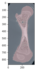
Application: The Femur Test, pt. 2
Ultimately, I’d like to use this on biological material. And everything is already in place.
We first get grays and positions:
# load the femur stack, extracted (i.e. cropped) from the full stack
femur = NP.array(TIF.imread('segments/d_exfemur.tiff'), dtype = NP.float64) / 2**bits
fmask = NP.array(TIF.imread('segments/b_exfemur.tiff') > 0, dtype = 'bool')

MPP.imshow(femur[:, femur.shape[1]//2, :], cmap = 'gray');
MPP.imshow(fmask[:, fmask.shape[1]//2, :], cmap = 'RdBu_r', alpha = 0.2);
MPP.gca().set_aspect('equal');
# positions and grays
positions = NP.stack(NP.where(fmask)).T
grays = NP.array([femur[pos[0], pos[1], pos[2]] for pos in positions])

positions = NP.array(positions, dtype = NP.float64) * voxel_edgelength
print (positions.shape, grays.shape)
(26233773, 3) (26233773,)
Here the two regression conversions:
# density regressions
mass_linear = LinInv(grays) * voxelvolume_m3
nonnan_linear = NP.logical_not(NP.isnan(mass_linear))

mass_expon = ExpInv(grays) * voxelvolume_m3
nonnan_expon = NP.logical_not(NP.isnan(mass_expon))

voxel_const = density_data.loc[density_data['material'].values == 'femur', 'measured_density']\
            .values[0] * voxelvolume_m3
mass_const = NP.ones((grays.shape[0],)) * voxel_const
And finally, the Inertia:
# Inertia calculation
actual_mass = 5.271*g
Itensor_linear_scaled, I_linear_scaled, Iaxes_linear_scaled = \
        DiagonalizedInertiaTensor(positions[nonnan_linear, :] \
                                   , mass_linear[nonnan_linear] * actual_mass / NP.nansum(mass_linear))
Itensor_expon_scaled, I_expon_scaled, Iaxes_expon_scaled = \
        DiagonalizedInertiaTensor(positions[nonnan_expon, :] \
                                     , mass_expon[nonnan_expon] * actual_mass / NP.nansum(mass_expon))

Itensor_const_scaled, I_const_scaled, _ = \
        DiagonalizedInertiaTensor(positions, mass_const * actual_mass / NP.nansum(mass_const))
26233773it [07:02, 62052.02it/s]
26233773it [06:57, 62822.50it/s]
26233773it [07:02, 62019.10it/s]
print ('linear:\t\t', NP.round(Itensor_linear_scaled.ravel()*1e9, 1))
print ('exponential:\t', NP.round(Itensor_expon_scaled.ravel()*1e9, 1))
print ('constant:\t', list(map(str,NP.round(Itensor_const_scaled.ravel()*1e9, 1))))
linear:		 [ 124.5    2.1   71.6    2.1  992.5    4.1   71.6    4.1 1004.8]
exponential:	 [ 127.6    1.3   75.3    1.3 1017.1    4.    75.3    4.  1028.7]
constant:	 ['130.8', '-0.3', '76.7', '-0.3', '1031.9', '4.1', '76.7', '4.1', '1042.3']
Both regressions give consistent results for inertia tensors, which is a good finding.
Although the reference data points would justify several, fundamentally different regression models, it does not matter much for the outcome.
Even if we convert with a constant (average) density, the inertia tensor is approximately correct. This makes me think that the segmentation (i.e. extracting the exact geometric shape of the object) is the more error-prone part of the procedure here.
Summary
Here again the lessons learned:
- CT artifacts matter, and should be minimized (e.g. by using filters and algorithmical corrections).
- Multiple regressions are plausible
- The exponential regression usually underestimates the voxel densities, but this can be rectified by scaling to the total mass of a segment.
- Both the linear regression and the scaled exponential regression can lead to consistent results that reproduce theoretical Inertia.
- Bone Mineral Density Phantoms are not well approximated as cylinders of homogeneous density.
Some practical issues to keep in mind, which I did not fully address:
- With all regression functions above, one can get negative masses (when segmenting air).
- Markers / high density areas produce artifacts.
- The Least Squares regression I used above has it’s flaws (e.g. sensitive to start values); I recommend using a probabilistic toolbox such as PyMC3 for the ability to enter all grey values and ultimately more robust results.
Acknowledgements
I involved a lot of people in this sidetrack, and I am thankful for their help and exchange. Those are:
Bjorn De Samber, Chris Broeckhoven, Jan Sijbers, Joaquim Sanctorum, Jonathan Brecko, Maja Mielke, Michael Fath, Van Thi Huyen Nguyen
… and of course my supervisors Chris, Peter and Sam.
Thank you all!
This will remain explorative, theoretical work for me. If you have any comments, do not hesitate to contact me. Thank you for feedback!
Update 20210414: Incorporated comments by Sam, e.g. included the “constant density” conversion.