You can download this notebook here.
For a student project, I have been playing around with stereo camera calibration. We have a set of cameras. The challenge is to obtain 3D kinematics by combining data from multiple views (i.e. simultaneously captured images from different perspectives).
Below, I document my attempts to relate the image space of the cameras (i.e. what is seen on each frame) to object space (i.e. the true 3D position of something).
Here is the usual extensive set of libraries I use below.
import numpy as NP # numeric operations
import pandas as PD # data organization

import cv2 as CV # open computer vision, i.e. image manipulation library

import sympy as SYM # symbolic python
import sympy.physics.mechanics as MECH # symbolic mechanics


import matplotlib as MP # plotting
import matplotlib.pyplot as MPP # plotting
from mpl_toolkits import mplot3d # 3D plots


# equal aspect for matplotlib 3D plots
# from https://stackoverflow.com/a/19248731
def AxisEqual3D(ax):
    extents = NP.array([getattr(ax, f'get_{dim}lim')() for dim in 'xyz'])
    sz = extents[:,1] - extents[:,0]
    centers = NP.mean(extents, axis=1)
    maxsize = max(abs(sz))
    r = maxsize/2
    for ctr, dim in zip(centers, 'xyz'):
        getattr(ax, f'set_{dim}lim')(ctr - r, ctr + r)
Ingredients
We have a set of consumer level GoPro “Hero 5” in the lab, three of which were attached to a rack of metal tubes. All were set to narrow field of view (to minimize fisheye lens distortion). Videos of resolution \(1280\times 720\) @ 240 fps were triggered with a remote control.
The same video settings were used to film a regular grid for undistortion (procedure as described here), which was applied to all the material used below.
The remote control sync was not accurate, which I found out only after calibration. I will use an extra audio clue in the future.
The setup is lightweight, mobile, and thus suited for field work.
Calibration Data
As a test calibration object, I grabbed a monitor box that was lying around in the office.
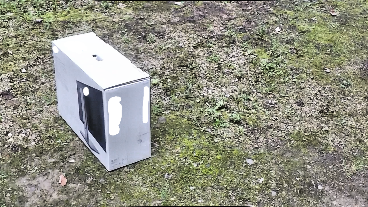
To get true 3D points, I prepared a 3D model of the box by photogrammetry.
Then, I used the “PickPoints” function in meshlab to get relative positions of the corner points and two extra landmarks on the box.
Taking simultaneous photos from the fixed cameras, I could also retrieve image points. Prior to calibration, those images were contrast enhanced and undistorted. All relevant images have to be prepared with the same procedure.
data = PD.read_csv('cam_calibration_data.csv', sep = ';').set_index('pt', inplace = False)
data
| x | y | z | u_1 | v_1 | u_2 | v_2 | u_4 | v_4 | |
|---|---|---|---|---|---|---|---|---|---|
| pt | |||||||||
| 0 | -0.235521 | 0.308646 | 0.101321 | 321.426491 | 111.782226 | 786.011187 | 252.220410 | 664.551136 | 65.475581 |
| 1 | -0.000698 | 0.311595 | 0.094717 | 180.229182 | 143.665489 | 710.098655 | 287.899300 | 537.777207 | 91.285842 |
| 2 | -0.004713 | -0.328370 | 0.089341 | 365.455760 | 315.986937 | 1073.719682 | 405.563724 | 814.857949 | 221.855397 |
| 3 | -0.236395 | -0.329500 | 0.092263 | 522.594701 | 272.716794 | 1129.894956 | 363.811832 | 946.186629 | 186.935632 |
| 4 | 0.005713 | 0.315304 | -0.349343 | 203.762067 | 394.935970 | 685.047519 | 527.023775 | 535.499831 | 356.979704 |
| 5 | 0.001885 | -0.331354 | -0.345600 | 379.879141 | 596.104179 | 1025.894787 | 662.148082 | 792.084189 | 524.746399 |
| 6 | -0.229327 | -0.330225 | -0.348522 | 524.872077 | 546.001908 | 1082.829186 | 606.731934 | 915.062491 | 479.198880 |
| 7 | 0.000000 | 0.000000 | 0.000000 | 266.010343 | 279.548921 | 868.755846 | 397.213346 | 656.200757 | 211.227643 |
| 8 | -0.132960 | 0.025250 | 0.097379 | 338.886374 | 191.490384 | 899.120859 | 313.709561 | 720.726409 | 125.446482 |
Note that object points are in meters, and should have a meaningful origin. Here are the images for download: cam1, cam2, cam4.
cams = [1,2,4]
images = {cam: CV.imread(f'images/cam{cam}.png', 1) for cam in cams}

# drawing its lines on left image
fig = MPP.figure(dpi = 300)

for nr, (cam, img) in enumerate(images.items()):
    ax = fig.add_subplot(1, len(images), nr+1, aspect = 'equal')
    ax.imshow(img[:, :, ::-1], origin = 'upper')

    pts = data.loc[:, [f'u_{cam}', f'v_{cam}']].values

    ax.scatter(pts[:, 0], pts[:, 1], s = 20 \
               , marker = '+', facecolor = 'r', edgecolor = '0' \
              , linewidth = 1, alpha = 0.6 \
              )

    ax.get_xaxis().set_visible(False)
    ax.set_yticks([])
    ax.set_xlabel(nr)

MPP.tight_layout()
MPP.show()
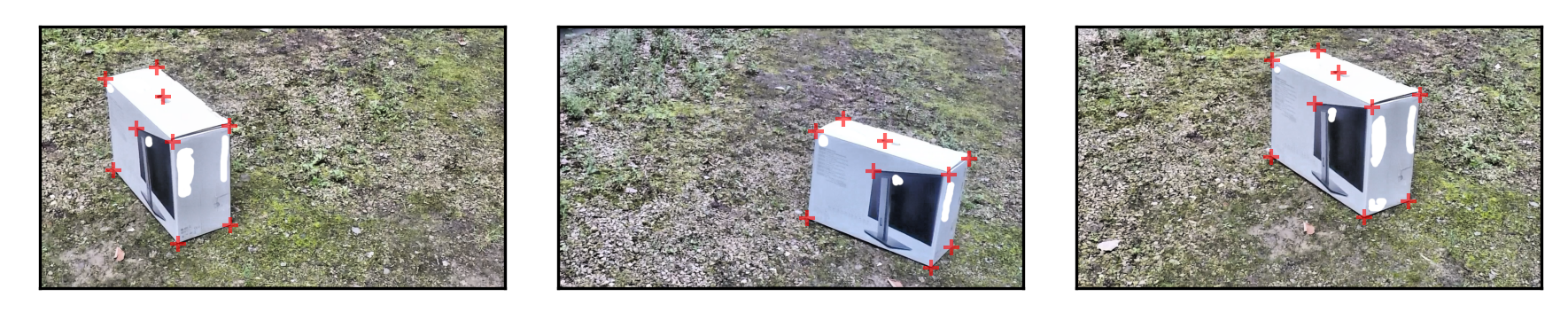
Of course, the points must always be labeled in the same order.
It would be better to use point labels as pandas data frame indices to make sure only matching points are associated.
In addition to the points on the images, the true 3D relation of the point is known:
data.loc[:, ['x', 'y', 'z']].T
| pt | 0 | 1 | 2 | 3 | 4 | 5 | 6 | 7 | 8 |
|---|---|---|---|---|---|---|---|---|---|
| x | -0.235521 | -0.000698 | -0.004713 | -0.236395 | 0.005713 | 0.001885 | -0.229327 | 0.0 | -0.132960 |
| y | 0.308646 | 0.311595 | -0.328370 | -0.329500 | 0.315304 | -0.331354 | -0.330225 | 0.0 | 0.025250 |
| z | 0.101321 | 0.094717 | 0.089341 | 0.092263 | -0.349343 | -0.345600 | -0.348522 | 0.0 | 0.097379 |
This can be used for calibration.
The Successful Attempt: DLT Calibration à la Argus/Kwon
My initial temptation was to go to openCV. For several reasons, these attempts failed (see below).
On the search for alternatives, I stumbled upon the argus toolbox from Ty Hedrick’s lab (Jackson et al., 2016). The toolbox had previously been recommended to me by a colleague, François Druelle.
I went through to the procedures referenced in the argus “theory” section. The authors implement algorithms collected in the Motion Analysis library of Young-Hoo Kwon. The Kwon3D website (Kwon, 2000) is a phenomenal resource for my research. I have already referenced the website in my force plate blog posts. I have now realized that my recent quest on solving inverse dynamics could have been facitilated by theory assembled on Kwon’s archives. And now, I also use the section on camera calibration via DLT for my purpose.
Theory
I start here with the naked maths. If that is of less interest to you, feel free to skip to the “numeric application” section below.
The website by Kwon excellently explains the DLT theory.
I will repeat it here in a sympy framework, using the same symbols.
# object space coordinates
x, y, z = SYM.symbols(f'x:z', real = True)
x0, y0, z0 = SYM.symbols(f'x_0, y_0, z_0', real = True)

# image space coordinates
u, v = SYM.symbols(f'u, v', real = True)
u0, v0, d = SYM.symbols(f'u_0, v_0, d', real = True)

# reference frame DCM
r = SYM.symbols('r_{1:4}{1:4}', real = True)
T_io = SYM.Matrix([r[:3],r[3:6],r[6:]]).T

# colinearity
c = SYM.symbols(f'c', real = True)
We require two reference frames. One is the object space, the other is the image plane (extended to 3D towards the focal point).
# object space
object_space = MECH.ReferenceFrame('O')

# image plane
image_plane = MECH.ReferenceFrame('I')
image_plane.orient(object_space, 'DCM', T_io)

# static
image_plane.set_ang_vel(object_space, 0)
image_plane.set_ang_acc(object_space, 0)

# transform between spaces
object_to_image = SYM.simplify(image_plane.dcm(object_space)) # frame_to.dcm(frame_from)
image_to_object = SYM.simplify(object_space.dcm(image_plane))

SYM.pprint(object_to_image)
⎡r_{1}{1}  r_{1}{2}  r_{1}{3}⎤
⎢                            ⎥
⎢r_{2}{1}  r_{2}{2}  r_{2}{3}⎥
⎢                            ⎥
⎣r_{3}{1}  r_{3}{2}  r_{3}{3}⎦
There are several points that can be located in either of the two reference frames. Most notably, the “projection center” (i.e. focal point) of the image can be located in both frames and connects the two.
### define the origins
# ... of the object space
origin = MECH.Point('Ω')

# of the image plane
origin_image = MECH.Point('ρ')

### points in the world
# object point in the world
obj_point = MECH.Point('ο')
obj_point.set_pos(origin, x * object_space.x + y * object_space.y + z * object_space.z)

### points in both worlds
# projection center: where all object point/projections meet
proj_center = MECH.Point('ν')
proj_center.set_pos(origin_image, u0 * image_plane.x + v0 * image_plane.y + d * image_plane.z)
proj_center.set_pos(origin, x0 * object_space.x + y0 * object_space.y + z0 * object_space.z)

### points in the image
# principal point (center of image plane; perpendicular axis through image plane and projection center)
principal_point = MECH.Point('π')
principal_point.set_pos(origin_image, u0 * image_plane.x + v0 * image_plane.y + 0 * image_plane.z)

# projection of the object point to the image plane
img_point = MECH.Point('ι')
img_point.set_pos(origin_image, u * image_plane.x + v * image_plane.y + 0 * image_plane.z)


### static: no movement of no point
for point in [origin, origin_image, obj_point, proj_center, principal_point, img_point]:
    point.set_vel(object_space, 0)
    point.set_acc(object_space, 0)
    point.set_vel(image_plane, 0)
    point.set_acc(image_plane, 0)
Take any vector which goes from the projection center to a true 3D point. Any such vector intersects the image plane at an image point. The vectors to the true point and to the plane are colinear, i.e. related by scalar multiplication.
This is the collinearity condition. It gives linear equations that relate the two spaces.
### vectors
A_o = obj_point.pos_from(proj_center).express(object_space)
B_i = img_point.pos_from(proj_center).express(image_plane)

A_i = A_o.express(image_plane)


equations = { coord: c*A_i.dot(coord) - B_i.dot(coord) \
              for coord in [image_plane.x, image_plane.y, image_plane.z] \
            }

equations
{I.x: c*(r_{1}{1}*(x - x_0) + r_{1}{2}*(y - y_0) + r_{1}{3}*(z - z_0)) - u + u_0,
 I.y: c*(r_{2}{1}*(x - x_0) + r_{2}{2}*(y - y_0) + r_{2}{3}*(z - z_0)) - v + v_0,
 I.z: c*(r_{3}{1}*(x - x_0) + r_{3}{2}*(y - y_0) + r_{3}{3}*(z - z_0)) + d}
Some values need to be substituted in, (i) to reduce dimensionality, (ii) to correct for an arbitrary scaling factor.
c_substitute = {c: SYM.solve(equations[image_plane.z], c)[0]}

λ_u, λ_v = SYM.symbols(f'λ_u, λ_v', real = True)
uv_substitutes = { \
                   (u-u0): λ_u * (u-u0) \
                 , (v-v0): λ_v * (v-v0) \
                 }

equations = { coord: equations[coord].subs(c_substitute).subs(uv_substitutes) \
              for coord in [image_plane.x, image_plane.y] \
            }
equations
{I.x: -d*(r_{1}{1}*(x - x_0) + r_{1}{2}*(y - y_0) + r_{1}{3}*(z - z_0))/(r_{3}{1}*x - r_{3}{1}*x_0 + r_{3}{2}*y - r_{3}{2}*y_0 + r_{3}{3}*z - r_{3}{3}*z_0) - λ_u*(u - u_0),
 I.y: -d*(r_{2}{1}*(x - x_0) + r_{2}{2}*(y - y_0) + r_{2}{3}*(z - z_0))/(r_{3}{1}*x - r_{3}{1}*x_0 + r_{3}{2}*y - r_{3}{2}*y_0 + r_{3}{3}*z - r_{3}{3}*z_0) - λ_v*(v - v_0)}
Finally, the resulting equations can be solved to get formulas for u and v (image coordinates) as a function of x, y and z (object coordinates).
u_eqn = SYM.Eq( u, SYM.simplify(SYM.solve(equations[image_plane.x], u)[0]).factor(x, y, z) )
v_eqn = SYM.Eq( v, SYM.simplify(SYM.solve(equations[image_plane.y], v)[0]).factor(x, y, z) )
solutions = [u_eqn, v_eqn]
for sol in solutions:
    SYM.pprint(sol)
    -(-d⋅r_{1}{1}⋅x₀ - d⋅r_{1}{2}⋅y₀ - d⋅r_{1}{3}⋅z₀ + r_{3}{1}⋅u₀⋅x₀⋅λᵤ + r_{
u = ──────────────────────────────────────────────────────────────────────────
                                                                    λᵤ⋅(r_{3}{

3}{2}⋅u₀⋅y₀⋅λᵤ + r_{3}{3}⋅u₀⋅z₀⋅λᵤ + x⋅(d⋅r_{1}{1} - r_{3}{1}⋅u₀⋅λᵤ) + y⋅(d⋅r_
──────────────────────────────────────────────────────────────────────────────
1}⋅x - r_{3}{1}⋅x₀ + r_{3}{2}⋅y - r_{3}{2}⋅y₀ + r_{3}{3}⋅z - r_{3}{3}⋅z₀)

{1}{2} - r_{3}{2}⋅u₀⋅λᵤ) + z⋅(d⋅r_{1}{3} - r_{3}{3}⋅u₀⋅λᵤ))
────────────────────────────────────────────────────────────

    -(-d⋅r_{2}{1}⋅x₀ - d⋅r_{2}{2}⋅y₀ - d⋅r_{2}{3}⋅z₀ + r_{3}{1}⋅v₀⋅x₀⋅λᵥ + r_{
v = ──────────────────────────────────────────────────────────────────────────
                                                                    λᵥ⋅(r_{3}{

3}{2}⋅v₀⋅y₀⋅λᵥ + r_{3}{3}⋅v₀⋅z₀⋅λᵥ + x⋅(d⋅r_{2}{1} - r_{3}{1}⋅v₀⋅λᵥ) + y⋅(d⋅r_
──────────────────────────────────────────────────────────────────────────────
1}⋅x - r_{3}{1}⋅x₀ + r_{3}{2}⋅y - r_{3}{2}⋅y₀ + r_{3}{3}⋅z - r_{3}{3}⋅z₀)

{2}{2} - r_{3}{2}⋅v₀⋅λᵥ) + z⋅(d⋅r_{2}{3} - r_{3}{3}⋅v₀⋅λᵥ))
────────────────────────────────────────────────────────────
You can convince yourself that this result is identical to the common DLT expression.
Sympy can perform what is called common subexpression elimination:
cse_replacements, dlt_terms = SYM.cse(solutions, symbols = SYM.utilities.iterables.numbered_symbols('L'))
SYM.pprint(dlt_terms)
⎡    -L₃⋅(L₀⋅L₇ + L₁⋅L₇ + L₂⋅L₇ - L₄⋅x₀ - L₅⋅y₀ - L₆⋅z₀ + x⋅(L₄ - L₇⋅r_{3}{1})
⎢u = ─────────────────────────────────────────────────────────────────────────
⎣                                                                λᵤ

 + y⋅(L₅ - L₇⋅r_{3}{2}) + z⋅(L₆ - L₇⋅r_{3}{3}))       -L₃⋅(L₀⋅L₁₁ + L₁⋅L₁₁ - L
────────────────────────────────────────────────, v = ────────────────────────


₁₀⋅z₀ + L₁₁⋅L₂ - L₈⋅x₀ - L₉⋅y₀ + x⋅(-L₁₁⋅r_{3}{1} + L₈) + y⋅(-L₁₁⋅r_{3}{2} + L
──────────────────────────────────────────────────────────────────────────────
                                         λᵥ

₉) + z⋅(L₁₀ - L₁₁⋅r_{3}{3})) ⎤
─────────────────────────────⎥
                             ⎦
However, this yields different parameters than the “guided” DLT parameters presented by Kwon.
The significant achievement of such DLT parameters is that one can build a system of linear equations to solve for the \(L_i\)’s.
Numeric Application
Multiplying by the RHS denominator, moving mixed terms to the right side and thereby isolating u, v results in such a system of linear equations.
A system of linear equations can be solved by linear algebra.
And if thinking of linear algebra raises your neck hair, rest assured that python will do the work for you.
Argus (Jackson et al., 2016) uses numpy.linalg.lstsq for this.
The function requires two matrices \(A\) and \(B\), for which we get \(L\) (the DLT parameters) from \(A L = B\).
To solve the systems, \(N\) points have to be known in both image and object space.
\(A\) is the coefficient matrix, shape \((2N \times 11)\). The number \(11\) comes from \(11\) \(L\) coefficients in the problem.
\( A = \begin{array}{c | ccccccccccc} i & 1 & 2 & 3 & 4 & 5 & 6 & 7 & 8 & 9 & 10 & 11 \\ \hline 2k & x_k & y_k & z_k & 1 & 0 & 0 & 0 & 0 & -u_k x_k & -u_k y_k & -u_k z_k \\ 2k+1 & 0 & 0 & 0 & 0 & x_k & y_k & z_k & 1 & -v_k x_k & -v_k y_k & -v_k z_k \end{array} \quad\quad \forall k \in \{0, N-1\} \)
And \(B\) is the dependent matrix:
\( B = \begin{array}{c | c} & \\ \hline 2k & u_k \\ 2k+1 & v_k \end{array} \quad\quad \forall k \in {0, N-1} \)
Then, computationally, \(\mid\mid B - A L \mid\mid\) is minimized by the least squares method.
Sounds fun? Here is the function, adapted from the argus code.
def SolveDLT(data, cam):
    # solve DLT for a camera
    # from N known points
    # adapted from https://github.com/kilmoretrout/argus_gui/blob/master/argus_gui/tools.py `solve_dlt`
    # input: a data frame with [x, y, z, u_i, v_i] columns where i is the camera index

    # coefficient matrix
    A = NP.zeros((data.shape[0] * 2, 11))

    # dependent variable
    B = NP.zeros((data.shape[0] * 2, 1))


    # fill the matrices
    for k, row in data.iterrows():
        A[2 * k, :3] = row[['x', 'y', 'z']].values
        A[2 * k, 3] = 1
        A[2 * k, 8:] = row[['x', 'y', 'z']].values * -row[f'u_{cam}']
        A[2 * k + 1, 4:7] = row[['x', 'y', 'z']].values
        A[2 * k + 1, 7] = 1
        A[2 * k + 1, 8:] = row[['x', 'y', 'z']].values * -row[f'v_{cam}']

        B[2 * k] = row[f'u_{cam}']
        B[2 * k + 1] = row[f'v_{cam}']

    # solve system of linear equations
    L = NP.linalg.lstsq(A, B, rcond=None)[0]
    return L.ravel()
Taking our data from above, the function can yield DLT parameters for the three cameras:
L = {cam: SolveDLT(data, cam = cam) for cam in cams}
L
{1: array([-7.03913782e+02, -2.04857500e+02, -1.03511822e+02,  2.65781236e+02,
         1.10530429e+02, -1.96650553e+02, -6.71888993e+02,  2.79123077e+02,
        -1.88877266e-01,  2.75455293e-01, -1.71605937e-01]),
 2: array([-5.55001628e+02, -3.98060092e+02, -5.05956178e+01,  8.68303335e+02,
         6.55700125e+01, -1.17488996e+02, -6.36343639e+02,  3.96662992e+02,
        -2.90184236e-01,  1.79093742e-01, -1.44750418e-01]),
 4: array([-7.29359405e+02, -2.20829579e+02, -9.97698632e+01,  6.56184624e+02,
         8.31303936e+01, -1.49535713e+02, -7.05594977e+02,  2.11502025e+02,
        -2.37017457e-01,  2.95065936e-01, -1.74821150e-01])}
To confirm the accuracy, we can project the 3D points to the image plane and check whether points match:
for cam in cams:

    for coord in ['u', 'v']:
        data[f'{coord}_{cam}_reco'] = 0

    for k, row in data.iterrows():
            data.loc[k, f'u_{cam}_reco'] = (NP.dot(L[cam][:3].T, row[['x', 'y', 'z']].values) + L[cam][3]) \
                                    / (NP.dot(L[cam][-3:].T, row[['x', 'y', 'z']].values) + 1.)
            data.loc[k, f'v_{cam}_reco'] = (NP.dot(L[cam][4:7].T, row[['x', 'y', 'z']].values) + L[cam][7]) \
                                    / (NP.dot(L[cam][-3:].T, row[['x', 'y', 'z']].values) + 1.)

data.loc[:, ['x', 'y', 'z', 'u_1', 'v_1', 'u_1_reco', 'v_1_reco']]
| x | y | z | u_1 | v_1 | u_1_reco | v_1_reco | |
|---|---|---|---|---|---|---|---|
| pt | |||||||
| 0 | -0.235521 | 0.308646 | 0.101321 | 321.426491 | 111.782226 | 321.775150 | 111.785891 |
| 1 | -0.000698 | 0.311595 | 0.094717 | 180.229182 | 143.665489 | 180.082729 | 144.087333 |
| 2 | -0.004713 | -0.328370 | 0.089341 | 365.455760 | 315.986937 | 365.453553 | 316.329381 |
| 3 | -0.236395 | -0.329500 | 0.092263 | 522.594701 | 272.716794 | 522.499640 | 272.692276 |
| 4 | 0.005713 | 0.315304 | -0.349343 | 203.762067 | 394.935970 | 203.651747 | 394.920945 |
| 5 | 0.001885 | -0.331354 | -0.345600 | 379.879141 | 596.104179 | 380.403750 | 595.960378 |
| 6 | -0.229327 | -0.330225 | -0.348522 | 524.872077 | 546.001908 | 524.553708 | 546.239586 |
| 7 | 0.000000 | 0.000000 | 0.000000 | 266.010343 | 279.548921 | 265.781236 | 279.123077 |
| 8 | -0.132960 | 0.025250 | 0.097379 | 338.886374 | 191.490384 | 338.916072 | 191.099186 |
fig = MPP.figure(dpi = 300)

for nr, cam in enumerate(cams):
    ax = fig.add_subplot(3, 1, nr+1, aspect = 'equal')

    ax.imshow(NP.mean(images[cam][:, :], axis = 2), cmap = 'gray', origin = 'upper')

    ax.scatter(  data[f'u_{cam}'].values \
               , data[f'v_{cam}'].values \
               , s = 40 \
               , marker = 'x' \
               , color = (0.2, 0.6, 0.2) \
               , alpha = 0.8 \
               , label = 'measured' \
              )
    ax.scatter(  data[f'u_{cam}_reco'].values \
               , data[f'v_{cam}_reco'].values \
               , s = 40 \
               , marker = '+' \
               , color = (0.6, 0.2, 0.2) \
               , alpha = 0.8 \
               , label = 'reconstructed' \
              )

    ax.legend(loc = 'best', fontsize = 4)

    ax.set_xticks([])
    ax.set_yticks([])
    ax.set_ylabel(cam)

fig.tight_layout()
MPP.show();
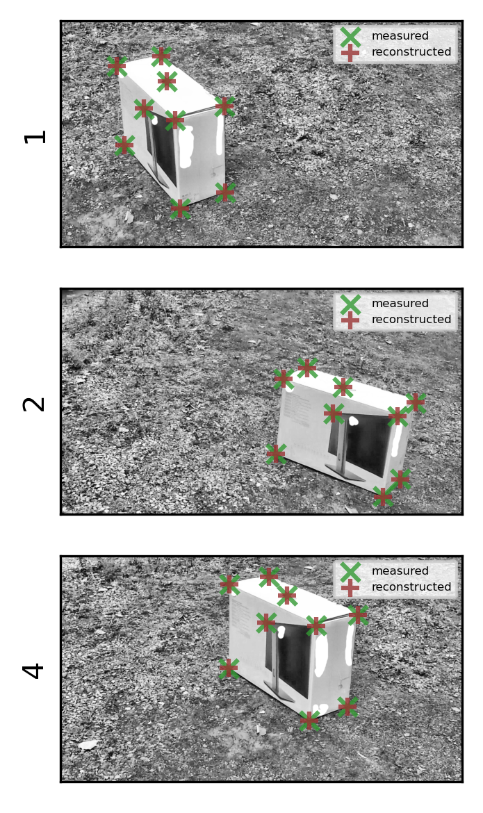
This check is trivial, but it looks like a match.
We’ll store the DLT parameters as a matrix.
# dlt: (number of cameras)x11 array of DLT coefficients
dlt = NP.stack([L[cam] for cam in cams], axis = 0)
dlt
array([[-7.03913782e+02, -2.04857500e+02, -1.03511822e+02,
         2.65781236e+02,  1.10530429e+02, -1.96650553e+02,
        -6.71888993e+02,  2.79123077e+02, -1.88877266e-01,
         2.75455293e-01, -1.71605937e-01],
       [-5.55001628e+02, -3.98060092e+02, -5.05956178e+01,
         8.68303335e+02,  6.55700125e+01, -1.17488996e+02,
        -6.36343639e+02,  3.96662992e+02, -2.90184236e-01,
         1.79093742e-01, -1.44750418e-01],
       [-7.29359405e+02, -2.20829579e+02, -9.97698632e+01,
         6.56184624e+02,  8.31303936e+01, -1.49535713e+02,
        -7.05594977e+02,  2.11502025e+02, -2.37017457e-01,
         2.95065936e-01, -1.74821150e-01]])
3D Point Reconstruction
When filming a calibration object, we know the true positions of points. Afterwards, when filming a scene, the goal is to take the observed image points and get their relative position in 3D, i.e. in “world coordinates”.
The argus code (Jackson et al., 2016) also contains a function for that.
def UVtoXYZ(pts, dlt):
    # retrieve Object Points (3D) from multiple perspective Image Points
    # adapted from https://github.com/kilmoretrout/argus_gui/blob/master/argus_gui/tools.py `uv_to_xyz`
    #     pts: (N x 2K) array of N 2D points for K cameras
    #          can be a single point over time, or multiple points in one scene
    #     dlt: (11 x K) array of DLT parameters
    # Adjusted because data points herein are undistorted prior to calculation

    # initialiye empty data array
    xyzs = NP.empty((len(pts), 3))
    xyzs[:] = NP.nan

    # for each point
    for i in range(len(pts)):
        uvs = list()
        # for each uv pair
        for j in range(len(pts[i]) // 2):
            # do we have a NaN pair?
            if not True in NP.isnan(pts[i, 2 * j:2 * (j + 1)]):
                # if not append the undistorted point and its camera number to the list
                uvs.append([pts[i, 2 * j:2 * (j + 1)], j])

        if len(uvs) > 1:
            # if we have at least 2 uv coordinates, setup the linear system
            A = NP.zeros((2 * len(uvs), 3))

            # assemble coefficient matrix of the linear system
            for k in range(len(uvs)):
                A[k] = NP.asarray([uvs[k][0][0] * dlt[uvs[k][1]][8] - dlt[uvs[k][1]][0],
                                   uvs[k][0][0] * dlt[uvs[k][1]][9] - dlt[uvs[k][1]][1],
                                   uvs[k][0][0] * dlt[uvs[k][1]][10] - dlt[uvs[k][1]][2]])
                A[k + 1] = NP.asarray([uvs[k][0][1] * dlt[uvs[k][1]][8] - dlt[uvs[k][1]][4],
                                       uvs[k][0][1] * dlt[uvs[k][1]][9] - dlt[uvs[k][1]][5],
                                       uvs[k][0][1] * dlt[uvs[k][1]][10] - dlt[uvs[k][1]][6]])

            # the dependent variables
            B = NP.zeros((2 * len(uvs), 1))
            for k in range(len(uvs)):
                B[k] = dlt[uvs[k][1]][3] - uvs[k][0][0]
                B[k + 1] = dlt[uvs[k][1]][7] - uvs[k][0][1]

            # solve it
            xyz = NP.linalg.lstsq(A, B, rcond=None)[0]
            # place in the proper frame
            xyzs[i] = xyz[:, 0]

    return xyzs
Here is how data can be assembled for this modified version:
reco = UVtoXYZ(data.loc[:, [f'{coord}_{cam}' for cam in cams for coord in ['u', 'v'] ]].values, dlt)
print (reco - data.loc[:, ['x', 'y', 'z']])
           x         y         z
pt
0   0.000953 -0.001926  0.001119
1   0.000111 -0.000483 -0.000105
2   0.000696 -0.002089  0.000875
3  -0.000479  0.000710 -0.000603
4  -0.000237  0.000237 -0.000447
5  -0.000047  0.001261 -0.000382
6   0.000397 -0.001256  0.000676
7   0.000072 -0.000616  0.000609
8  -0.001467  0.004175 -0.001740
And because those are just the calibration points, we can check whether the positions match.
pts = data.loc[:, ['x', 'y', 'z']].values
fig = MPP.figure(dpi = 300)
ax = fig.add_subplot(1,1,1,projection='3d', aspect = 'auto')

edge_kwargs = dict( \
                  lw = 0.5 \
                , alpha = 0.8 \
                , zorder = 0 \
                , label = None \
                  )

for edge in [[0,1], [1,2], [2,3], [3,0], [4,5], [5,6], [4,1], [5,2], [6,3]]:
    ax.plot(  reco[edge, 0] \
            , reco[edge, 1] \
            , reco[edge, 2] \
            , color = 'k' \
            , ls = '-' \
            , **edge_kwargs
              )

    ax.plot(  pts[edge, 0] \
            , pts[edge, 1] \
            , pts[edge, 2] \
            , color = '0.9' \
            , ls = ':' \
            , **edge_kwargs
              )


ax.scatter(  pts[:, 0] \
           , pts[:, 1] \
           , pts[:, 2] \
           , s = 16 \
           , marker = 'o' \
           , color = (0.2, 0.6, 0.2) \
           , alpha = 0.8 \
           , zorder = 10 \
           , label = 'true points' \
          )

ax.scatter(  reco[:, 0] \
           , reco[:, 1] \
           , reco[:, 2] \
           , s = 32 \
           , marker = '+' \
           , linewidth = 0.5 \
           , color = (0.6, 0.2, 0.6) \
           , alpha = 0.8 \
           , zorder = 20 \
           , label = 'reconstructed points' \
          )


ax.legend(loc = 1, fontsize = 4)


ax.set_xlabel('x')
ax.set_ylabel('y')
ax.set_zlabel('z')

ax.view_init(30, -20)

AxisEqual3D(ax)

MPP.show();
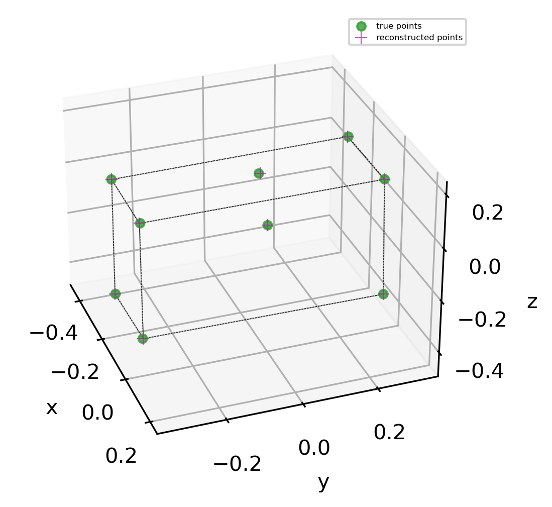
… and they do, it is a box!
It remains too be seen whether a space far from the calibration object can be well reconstructed.
Applied Example: Dog Video
When testing our setup, two kind shepards with their dogs passed by. (Our university is keeping sheep on the green areas of our campus.)
They allowed us to follow to the meadow and get a few shots of the animals.
Here is one, in real time, from multiple perspectives:
I tracked one stride cycle of the accelerating dog.
Because I have three cameras, I can reconstruct 3D data with two of them, and project that into the third camera (using a modified dlt_inverse from argus).
Purple are the tracked points, red are the reprojections (slowed down 10x):
I will have to find out where the offset comes from; one reason might be that the calibration videos were not in sync.
Apart from that, the data looks reasonable. But…
…let’s look at the 3D data from all cameras:
The lateral perspective seems okay. However, the depth is not well recovered. This is only in part due to the lacking contrast on some landmarks (e.g. the knee), as can be seen from the well-defined snout point. The other problem is the way I arranged my cameras (flat, next to each other).
I’ll have to improve on that. One way is more accurate calibration. The other is optimization of the camera distance and angles. Noteworthy, the problem is general: if the view directions of cameras pointing at the same scene are at a low relative angle, i.e. if the focal planes are relatively parallel, then the depth is less accurate than the other spatial dimensions. This inaccuracy is not captured by calculating the reprojection error.
Still, getting accurate 3D data this way would be appealing: units are in meters and 3D, so accurate angles and speeds can be determined. There is certainly room for improvement.
Probabilistic DLT
Does the depth inaccuracy come from inaccurate calibration, or from inaccurate tracking?
To tackle this question, one can use probabilistic modeling of the DLT parameters.
Luckily, the formula above can easily be brought to a probabilistic context. Let’s bring in some additional libraries.
import pymc3 as PM

import theano as TH
import theano.tensor as TT
Prepare the matrices as before:
def PrepareDLTData(cam_data):
    # prepare linear equations in matrix form from data of one camera
    # adapted from https://github.com/kilmoretrout/argus_gui/blob/master/argus_gui/tools.py `solve_dlt`
    # input: a data frame with [x, y, z, u, v] columns

    # coefficient matrix
    A = NP.zeros((cam_data.shape[0] * 2, 11))

    # dependent variable
    B = NP.zeros((cam_data.shape[0] * 2, 1))


    # fill the matrices
    for k, row in cam_data.iterrows():
        A[2 * k, :3] = row[['x', 'y', 'z']].values
        A[2 * k, 3] = 1
        A[2 * k, 8:] = row[['x', 'y', 'z']].values * -row['u']
        A[2 * k + 1, 4:7] = row[['x', 'y', 'z']].values
        A[2 * k + 1, 7] = 1
        A[2 * k + 1, 8:] = row[['x', 'y', 'z']].values * -row['v']

        B[2 * k] = row['u']
        B[2 * k + 1] = row['v']

    return A, B
Here comes the actual data:
cams = [1, 2, 4]
n_cams = len(cams)
A = {}
B = {}
Λ = {}

for cam in cams:
    A[cam], B[cam] = PrepareDLTData(data.copy() \
                                    .loc[:, ['x', 'y', 'z', f'u_{cam}', f'v_{cam}']] \
                                    .rename(columns = {f'u_{cam}': 'u', f'v_{cam}': 'v'} \
                                           , inplace = False) \
                                   )

    Λ[cam] = NP.linalg.lstsq(A[cam], B[cam], rcond=None)[0] # to get accurate priors


print (A[1].shape, Λ[1].shape)
print (NP.sum(NP.abs((A[1] @ Λ[1]).ravel() - B[1].T.ravel())))
(A[1] @ Λ[1]).T
(18, 11) (11, 1)
3.855946132496541


array([[321.8142397 , 111.78630141, 180.07251953, 144.11673908,
        365.45378411, 316.2934613 , 522.50552844, 272.69379468,
        203.63567058, 394.91875521, 380.38679315, 595.96502565,
        524.54983622, 546.24247655, 265.78123573, 279.12307693,
        338.91652818, 191.09317816]])
The model is equivaltent to what was fed to lstsq above.
However, we have the flexibility to use robust regression by making the posterior distribution StudentT.
Hence, the result will be more robust to outliers, without the need for a RANSAC (Random sample consensus).
def ProbabilisticDLTModel(A, B, L):

    with PM.Model() as model:

        # the DLT parameters L
        λ = PM.Normal('λ', mu = L.reshape([-1,1]), sd = 2*NP.std(L), shape = (11,1))

        # matrix multiplication
        # A must be a theano tensor
        estimator = TH.shared(A) @ λ

        # model residual
        residual = PM.HalfCauchy('ε', 10.)

        # Students T degrees of freedom
        dof = PM.HalfNormal('η', 10.)

        # posterior distribution/"likelihood"
        posterior = PM.StudentT(  'post' \
                                , nu = dof \
                                , mu = estimator \
                                , sd = residual \
                                , observed = B \
                               )
    # sampling:
        trace = PM.sample(draws = 2**10, chains = 2**3, cores = 2**2, target_accept = 0.906)

    return model, trace
Once the model is prepared, the distributions can be fit to the data.
models = {}
traces = {}
for cam in cams:
    print ('#'*4, f' Creating DLT model for cam {cam} ', '#'*4)
    models[cam], traces[cam] = ProbabilisticDLTModel(A[cam], B[cam], Λ[cam])

    print()
####  Creating DLT model for cam 1  ####


Auto-assigning NUTS sampler...
Initializing NUTS using jitter+adapt_diag...
Multiprocess sampling (8 chains in 4 jobs)
NUTS: [η, ε, λ]
Sampling 8 chains, 0 divergences: 100%|██████████| 12192/12192 [00:26<00:00, 468.71draws/s]
The number of effective samples is smaller than 10% for some parameters.


####  Creating DLT model for cam 2  ####


Auto-assigning NUTS sampler...
Initializing NUTS using jitter+adapt_diag...
Multiprocess sampling (8 chains in 4 jobs)
NUTS: [η, ε, λ]
Sampling 8 chains, 0 divergences: 100%|██████████| 12192/12192 [00:37<00:00, 327.34draws/s]
The acceptance probability does not match the target. It is 0.8449641766015696, but should be close to 0.906. Try to increase the number of tuning steps.
The acceptance probability does not match the target. It is 0.7517996349827041, but should be close to 0.906. Try to increase the number of tuning steps.
The number of effective samples is smaller than 25% for some parameters.


####  Creating DLT model for cam 4  ####


Auto-assigning NUTS sampler...
Initializing NUTS using jitter+adapt_diag...
Multiprocess sampling (8 chains in 4 jobs)
NUTS: [η, ε, λ]
Sampling 8 chains, 0 divergences: 100%|██████████| 12192/12192 [00:37<00:00, 326.80draws/s]
The number of effective samples is smaller than 25% for some parameters.
And here are the results, example model 1:
PM.traceplot(traces[1], combined = True, var_names = ['ε', 'η']);
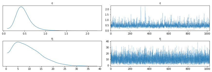
Hmmm… that Student does not look very normal.
We can get all the \(L_i\)s for each camera (\(\lambda\) here):
summary = PM.summary(traces[1])
summary
| mean | sd | hpd_3% | hpd_97% | mcse_mean | mcse_sd | ess_mean | ess_sd | ess_bulk | ess_tail | r_hat | |
|---|---|---|---|---|---|---|---|---|---|---|---|
| λ[0,0] | -703.478 | 5.148 | -713.327 | -693.761 | 0.109 | 0.077 | 2241.0 | 2241.0 | 2191.0 | 1496.0 | 1.00 |
| λ[1,0] | -204.950 | 1.743 | -208.108 | -201.676 | 0.030 | 0.021 | 3456.0 | 3449.0 | 3603.0 | 3559.0 | 1.00 |
| λ[2,0] | -103.390 | 2.881 | -108.717 | -97.805 | 0.051 | 0.036 | 3138.0 | 3138.0 | 3135.0 | 3348.0 | 1.00 |
| λ[3,0] | 265.808 | 0.282 | 265.249 | 266.306 | 0.004 | 0.003 | 4498.0 | 4498.0 | 4432.0 | 4508.0 | 1.00 |
| λ[4,0] | 110.696 | 3.743 | 103.891 | 118.065 | 0.073 | 0.052 | 2599.0 | 2599.0 | 2548.0 | 2141.0 | 1.00 |
| λ[5,0] | -196.683 | 1.656 | -199.680 | -193.472 | 0.028 | 0.020 | 3612.0 | 3602.0 | 3793.0 | 3767.0 | 1.00 |
| λ[6,0] | -671.693 | 3.635 | -678.613 | -665.013 | 0.067 | 0.047 | 2930.0 | 2930.0 | 2887.0 | 3407.0 | 1.00 |
| λ[7,0] | 279.143 | 0.299 | 278.571 | 279.699 | 0.004 | 0.003 | 5299.0 | 5298.0 | 5166.0 | 4335.0 | 1.00 |
| λ[8,0] | -0.188 | 0.011 | -0.206 | -0.165 | 0.000 | 0.000 | 2267.0 | 2267.0 | 2222.0 | 1241.0 | 1.00 |
| λ[9,0] | 0.275 | 0.005 | 0.265 | 0.285 | 0.000 | 0.000 | 2812.0 | 2812.0 | 2913.0 | 3178.0 | 1.00 |
| λ[10,0] | -0.171 | 0.008 | -0.186 | -0.157 | 0.000 | 0.000 | 2994.0 | 2994.0 | 3037.0 | 3299.0 | 1.00 |
| ε | 0.473 | 0.183 | 0.200 | 0.852 | 0.006 | 0.004 | 1080.0 | 1080.0 | 778.0 | 358.0 | 1.01 |
| η | 9.496 | 5.839 | 0.842 | 19.973 | 0.100 | 0.071 | 3411.0 | 3411.0 | 1344.0 | 364.0 | 1.01 |
Results match what we found with least squares:
print ('\n'.join(map(str, list(zip(map(lambda x: round(x[0], 3), Λ[1][:]), summary['mean'].values[:11])))))
(-703.914, -703.478)
(-204.858, -204.95)
(-103.512, -103.39)
(265.781, 265.808)
(110.53, 110.696)
(-196.651, -196.683)
(-671.889, -671.693)
(279.123, 279.143)
(-0.189, -0.188)
(0.275, 0.275)
(-0.172, -0.171)
Finally, and most importantly, instead of using only one fixed value for each \(L_i\), we can sample the posterior distribution to get some values and thereby find out how our point calculations vary.
n_samples = 1000
post_samples = {cam: NP.squeeze(PM.sample_posterior_predictive( \
                                traces[cam] \
                              , var_names = ['λ'] \
                              , samples = n_samples \
                              , model = models[cam] \
                              , progressbar = True \
                             )['λ']) \
                for cam in cams }
post_samples[1].shape
/usr/lib/python3.8/site-packages/pymc3/sampling.py:1246: UserWarning: samples parameter is smaller than nchains times ndraws, some draws and/or chains may not be represented in the returned posterior predictive sample
  warnings.warn(
100%|██████████| 1000/1000 [00:00<00:00, 29193.81it/s]
100%|██████████| 1000/1000 [00:00<00:00, 27780.16it/s]
100%|██████████| 1000/1000 [00:00<00:00, 31130.95it/s]


(1000, 11)
There we have many many samples for \(L\)-values of each camera. Let’s take a single measurement of \((u_1, v_1, u_2, v_2, u_4, v_4)\) and see how the variation in \(L\) affects the \((x, y, z)\) reconstruction.
We’ll take a regular grid of points in object space.
grid_pts = [NP.linspace(-1.0, 1.0, 5, endpoint = True).ravel()]*3
xyz = NP.stack(list(map(NP.ravel, NP.meshgrid(*grid_pts))), axis = 1)
xyz.shape
(125, 3)
We’ll need another function from the argus_gui code:
def DLTInverse(L, xyz):

    uv = NP.zeros((len(xyz), 2))
    for k in range(uv.shape[0]):
        u = (NP.dot(L[:3].T, xyz[k]) + L[3]) / (NP.dot(L[-3:].T, xyz[k]) + 1.)
        v = (NP.dot(L[4:7].T, xyz[k]) + L[7]) / (NP.dot(L[-3:].T, xyz[k]) + 1.)
        uv[k] = [u, v]
    return uv

uv = NP.concatenate([DLTInverse(L[cam], xyz) for cam in cams], axis = 1)
uv.shape
(125, 6)
And then we can convert the uvs back to xyzs with variable Ls, thereby measuring the inaccuracy that results from our DLT parameters.
reco = NP.stack( \
             [ \
             UVtoXYZ(uv, NP.stack([post_samples[cam][i, :] for cam in cams], axis = 0)) \
             for i in range(n_samples) \
             ] \
             , axis = 2) \


reco_centered = NP.concatenate([reco[:, :, r] - xyz for r in range(reco.shape[2])], axis = 0)
reco_stacked = NP.concatenate([reco[:, :, r] for r in range(reco.shape[2])], axis = 0)

span = NP.array([NP.diff(NP.percentile(reco[:, i], [5, 95])) for i in range(reco.shape[1])]).ravel()
print ('space spanned by the test points:', span)
print (' standard deviation about each point:', reco_centered.std(axis = 0))
space spanned by the test points: [2.0214302  2.0318401  2.02179291]
 standard deviation about each point: [0.01706024 0.03142076 0.01727276]
The inaccuracy from calibration in a \(2\ m^3\) volume is in the order of \(0.05\ m\). It drastically increases when moving away from the calibration object (\(0.5\ m\), i.e. factor \(10\), for \(5\ m^3\) cube). Hence, at least part of the inaccuracy problem in our case stems from the fact that the calibration object did not fill the calibration space. Most notably, in was at a different depth than the animal recording.
I conclude that target area (especially distance) has to be taken into account, and calibration should happen at approximately the same position from the cameras as recording, filling the field of view as good as possible.
The utility of probabilistic modeling and posterior sampling cannot be emphasized enough. It is well known for statistics, but it is equally useful to quantify the uncertainty in experimental measurements. Do not hesitate to try it yourself!
As a start, you might want to check this recent youtube tutorial. Or, of course, follow the book and lecture by Richard McElreath which I’ve repeatedly linked on my blog.
OpenCV Attempts: Epipolar Geometry
The DLT reconstruction exemplified above is just scratching on the surface of stereo vision theory, or epipolar geometry. There are a lot of resources that I found relevant for diving deeper:
-
Lecture by Rich Radke https://www.youtube.com/watch?v=QzYn0OPO0Yw
-
Lecture by Cyrill Stachniss https://www.youtube.com/watch?v=cLeF-KNHgwU
-
OpenCV documentation https://docs.opencv.org/master/d9/d0c/group__calib3d.html
-
Argus documentation http://argus.web.unc.edu/formal-methods-and-definitions
This might help you to build a basic set of vocabulary, containing for example terms as
- camera matrix ←
CV.calibrateCamera - distortion coefficients ←
CV.calibrateCamera - fundamental matrix ←
CV.findFundamentalMat - essential matrix ←
CV.findEssentialMat - epilines = epipolar lines ←
CV.computeCorrespondEpilines
The openCV functions next to it are some of many functions related to that topic.
I experienced some trouble with openCV because my workflow deviates from the supposed calibration.
The trouble arose because (i) my images were undistorted prior to processing, and (ii) I used a box instead of multiple views of a chessboard.
But I also noted that the openCV error messages are not very instructive. For example, when trying to calibrate from a single scene, one might encounter the error
src\calibration.cpp:3110: error: (-210) objectPoints should contain vector of vectors of points of type Point3f in function cv::collectCalibrationData.
In my case, this could be solved by adding a fake dimension to the object_points by wrapping it in a list [object_points].
Another example are data types, which should always be NP.float32 to avoid openCV chaos.
Nevertheless, openCV is probably the most comprehensive image processing library out there, and when you understand the logic behind it and are willing to scan through the raw code, it will doubtlessly be useful.
Epiline Calculation
Here is one example of how to use openCV to get epilines in corresponding images of different perspective.
One can use the fundamental matrix to relate the images, without even knowing the absolute positions of the calibration object.
When displayed during tracking, epilines can result in more accurate results on low-contrast landmarks.
The steps to get epilines are as follows:
- digitize points on calibration images of both cameras
- calculate the fundamental matrix with
CV.findFundamentalMat - compute “epilines” for arbitrary points of interest with
CV.computeCorrespondEpilines
# get two arrays of calibration point coordinates
points = {cam: data.loc[:, [f'{coord}_{cam}' for coord in ['u', 'v'] ]].values \
          for cam in cams }

# calculate fundamental matrix
fundamental_matrix = {(cam1, cam2): CV.findFundamentalMat(points[cam1], points[cam2], CV.FM_LMEDS)[0] \
                      for cam1 in cams for cam2 in cams \
                     }
The epilines can be displayed on the images:
colors =[tuple(NP.random.randint(150,255,3).tolist()) for _ in range(points[1].shape[0])]

cross_images = { cam: images[cam].copy()//2 for cam in cams } # darkened images

# loop cameras
for cam in cams:
    pts = points[cam]
    img = cross_images[cam]

    if len(img.shape) == 3:
        r,c,ch = img.shape
        img = img // 2
    else:
        r,c = img.shape
        img = CV.cvtColor(img,CV.COLOR_GRAY2BGR) // 2

    # loop the other cameras
    for crosscam in cams:
        if cam == crosscam:
            continue

        funmat = fundamental_matrix[(cam, crosscam)]

        # add a line for each other image
        lines = CV.computeCorrespondEpilines(points[crosscam].reshape(-1,1,2), 2, funmat).reshape(-1,3)
        #print (lines)

        for count, r in enumerate(lines):
            x0,y0 = [0, -r[2]/r[1] ]
            x1,y1 = [c, -(r[2]+r[0]*c)/r[1] ]

            # superimpose line on the image
            img = CV.line(img, (int(x0),int(y0)), (int(x1),int(y1)), colors[count],1)

    # add a point for the current image

    for count, pt1 in enumerate(pts):
        img = CV.circle(img,tuple(NP.array(pt1, dtype = int)),5,colors[count],-1)

    cross_images[cam] = img
Here is the result:
# drawing its lines on left image
fig = MPP.figure(dpi = 300)

for nr, cam in enumerate(cams):
    ax = fig.add_subplot(len(cams), 1, nr+1)
    ax.imshow(cross_images[cam], cmap = 'gray')

    ax.get_xaxis().set_visible(False)
    ax.set_yticks([])
    ax.set_ylabel(cam)

MPP.tight_layout()
MPP.show()
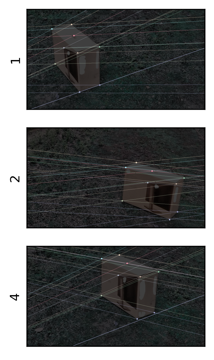
Looking closely, one can see that some lines are off - again the calibration settings might not be ideal.
OpenCV Camera Calibration
As mentioned above, openCV is versatile, but also bloated, which is the typical fate of complex code.
I ultimately failed to established my desired workflow in that toolbox due to trouble with CV.calibrateCamera.
I used it as follows:
GetCMat = lambda foc, cx, cy: NP.array([[foc, 0, cx], [0, foc, cy], [0, 0, 1]], dtype = NP.float32)
GetDistorts = lambda k_vec: NP.array(k_vec, dtype = NP.float32)

CV.calibrateCamera(object_points \
                 , image_points \
                 , (1280, 720) # resolution \
                 , cameraMatrix = GetCMat(*start_values[:3]) \
                 , distCoeffs = GetDistorts(start_values[3:]) \
                 , flags = CV.CALIB_USE_INTRINSIC_GUESS \
                 )
The presence of start_values therein indicates that I used a manual layer of optimization (scipy.optimize) to get the correct camera matrix and distortion parameters.
This is highly confusing to me: in my opinion, these parameters should be deterministic.
However, in openCV, they depend on the start values I give, and how they depend could not even be reproducibly inferred with Nelder-Mead algorithm.
At that point, I researched more and turned to DLT as documented by Argus and Kwon.
Digression: Photogrammetry
Fundamental matrix extraction and epiline generation worked with a fundamental matrix that was calculated from known, manually digitized points.
In contrast, openCV also offers functions that find keypoints automatically, turns them into descriptors, and matches. Some code to give you a direction:
# Initiate ORB detector
orb = cv.ORB_create(32)

# find the keypoints and descriptors with ORB
kp1, des1 = orb.detectAndCompute(img1,None)
kp2, des2 = orb.detectAndCompute(img2,None)

# brute force matching
bf = cv.BFMatcher(cv.NORM_HAMMING, crossCheck = True)
matches = bf.match(des1, des2)

# Alternative: FLANN/K nearest neighbors (knn)
index_params = dict(algorithm = 1, trees = 5)
search_params = dict(checks=50) # or pass empty dictionary
flann = cv.FlannBasedMatcher(index_params, search_params)

# match:
matches = flann.knnMatch(np.float32(des1),np.float32(des2),k=2)
This is the heart of Photogrammetry, so feel free to create your own photogrammetry workflow with it.
update 2021/02: More details on Photogrammetry in this blog post.
Summary
Above, I demonstrated how to calibrate an array of cameras in fixed relative position to get 3D data. Accuracy was limited with the simple calibration object I used. But I demonstrated how probabilistic programming and posterior sampling can give you a feel for the accuracy of your personal calibration procedure. Besides that, temporal sync and camera arrangement left room for improvement.
I also pointed out some directions for interested readers to instead use the much more potent openCV library, with all the pitfalls it contains.
I like the Argus slogan, 3D for the people, and hope that I could contribute my part with this little tutorial. It turns out that it is not that trivial to capture our 3D world in 2D images. But thanks to web documentation and great open source projects, there is hope!
References
-
Jackson, Brandon E and Evangelista, Dennis J and Ray, Dylan D and Hedrick, Tyson L (2016). 3D for the people: multi-camera motion capture in the field with consumer-grade cameras and open source software. Biology Open 5: 1334-1342; https://doi.org/10.1242/bio.018713. http://argus.web.unc.edu, accessed 2020/08/01
-
Kwon, Young-Hoo (2000). Direct Linear Transformation (DLT). Kwon3D Theoretical Foundation. http://kwon3d.com/theories.html, accessed 2020/08/01
Further reading:
-
Abdel-Aziz, Y.I., & Karara, H.M. (1971). Direct linear transformation from comparator coordinates into object space coordinates in close-range photogrammetry. Proceedings of the Symposium on Close-Range Photogrammetry (pp. 1-18). Falls Church, VA: American Society of Photogrammetry.
-
Miller, N.R., Shapiro, R., & McLaughlin, T.M. (1980). A technique for obtaining spatial kinematic parameters of segments of biomechanical systems from cinematographic data. J. Biomech 13, 535-547.
UPDATE 2020/08/04: added probabilistic calibration section