Force Plates IV

Calibration of Sensor Depth

Falk Mielke, University of Antwerp, July 17, 2019

forces experiments calibration

You can download this notebook here.

This is one part of a series of blog posts on Force Plates.

Sensor Depth Calibration

Recall that my original goal was to use contact sockets to improve the probability of recording single limb forces of quadruped vertebrates that locomote. This looks as follows:

Now because we add padding, i.e. the socked that increases the height of the contact surface above the internal sensor, the situation of the force recording changes. Whereas the forces stay the same (given that the socket itself is perfectly solid and inelastic), the moments are transferred via the additional stiff element.

But what is the value for padding that has to be set in the kistler software? Should it be found on calibration sheets that were long lost? Does Kistler software know, from the serial number of the force plate, what the basic padding is and transform all data to “surface level” values? Last but not least: our force plate had a mounting adapter (metal plate with screw holes) attached on top. Is that included, or not?

So many questions, one answer: calibration. Let’s find out definitely how deep below the surface the piezo sensors are located.

I have previously demonstrated how to get the right force units out of a raw voltage recording, which required the calibration of a uniform conversion factor. This unit conversion is no prerequisite for what follows.

Here, I will demonstrate how to regress the contact point = centre of pressure (CoP). In principle, the calculation is simple, but it requires one of the most relevant tools of force measurement.

Here is a collection of python libraries used below, as well as some helper functions.

#######################################################################
### Libraries                                                       ###
#######################################################################
# data management
import numpy as NP
import pandas as PD
import scipy.stats as STATS

PD.set_option('precision', 5) # for display

# symbolic maths
import sympy as SYM
import sympy.physics.mechanics as MECH
from sympy.matrices import rot_axis3 as ROT3

# plots and graphics
import matplotlib as MP
import matplotlib.pyplot as MPP
from IPython.core.display import SVG

%matplotlib inline

# formula printing
SYM.init_printing(use_latex=False)

# vector (de)composition helpers
VectorComponents = lambda vec, rf: [vec.dot(rf.x), vec.dot(rf.y), vec.dot(rf.z)]
MakeVector = lambda components, coords, n = 3: sum(NP.multiply(components[:n], coords[:n]))
ChangeAFrame = lambda vec, rf_old, rf_new: MakeVector(VectorComponents(vec, rf_old), [rf_new.x, rf_new.y, rf_new.z])

SmallAngleApprox = lambda ang: [(SYM.sin(ang), ang), (SYM.cos(ang), 1), (SYM.tan(ang), ang)]

def PrintSolution(solution_dict):
    # print and substitute in known values
    for param, eqn in solution_dict.items():
        print ('\n', '_'*20)
        print (param)
        print ('_'*20)
        SYM.pprint(eqn.subs(fp_dimensions))

What Has Three Legs and a Rectum on the Top Side?

… a drum stool.

This old joke is based on the observation that drum seats are essentially tripods. For our purpose, let’s take away the drummer (just because our kind can’t sit still). Tripods are very useful, and every student seriously aiming at force recordings should have one.

Tripods are part of regular photo equipment, drumming equipment, etc. But most importantly: tripods are well determined systems due to their symmetry. The reasons why tripods are so useful are that they have a predictable horizontal force component in the static case, that the leg angle and length can be adjusted (and with it the horizontal force), and that mounting some extra weight on top is easy.

For testing, I put one leg of a tripod of a given mass on the force plate. In fact, the mass does not matter much, only that its legs are fixed and remain fixed during the recording.

I did this with the Kistler BioWare software, but it is independent of DAQ/Computer assembly. Kistler software allows the export of the desired parameters, but I was not sure whether I entered everything correctly. Since I did not know the padding height (\(az_0\) in Kistler terminology; has to be entered in the software), I thought it’s worth comparing theoretical calculations, Kistler output, and my own conversion.

Fun fact: one can order support by a Kistler technician, who comes to help you with the software settings at a daily rate of approximately 1800.-EUR. Must be a clever guy. But enough Kistler bashing for now. Always know that you can have me for 999,-EUR (plus travel expenses).

Below an overview of the test setup.

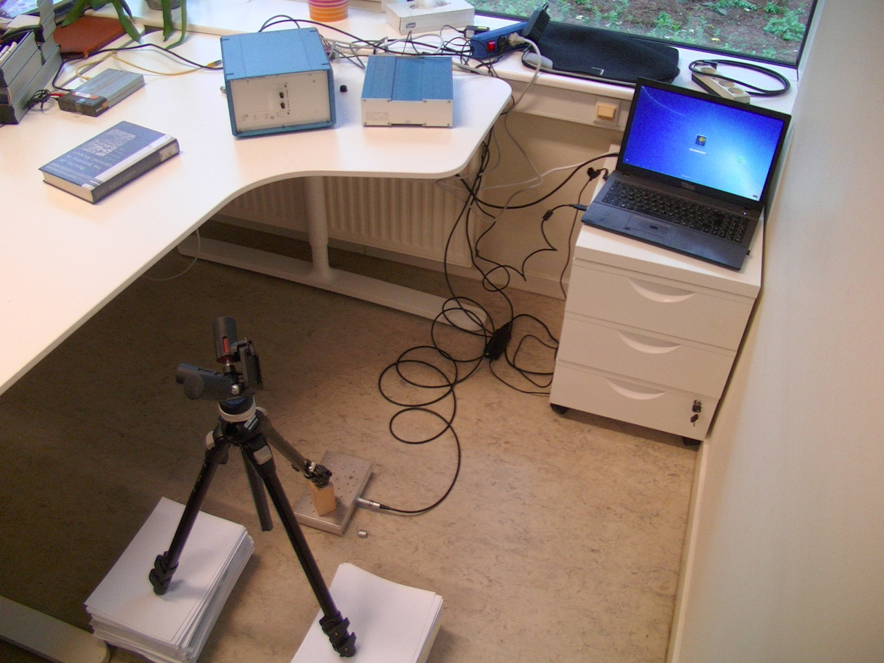
This was one of my first installations - today, I consider it more a kind of art than relevant measurement. I had carefully measured tripod angles, weighted the tripod, had meticulously piled books and papers to level out the feet, fixed a wooden socket on the force plate, and even made sure that all legs of the tripod get the same share of its weight.

So what do you guess is irrelevant in this setting (excluding the measurement tools)?

\(\ldots\)

Correct! All except the tripod. I learned a lot with these measurements.

What can benefit our purpose though is a point tip on one of the legs. I tend to tape screws to it - simple and efficient. The pointier, the better, and it should be tightly fixed, but careful not to hurt yourself or anyone.

The Tripod Trick

You are already able to calculate moments and contact points from the raw Kistler output. Put the tripod with one pointy leg on the force plate. Imagine you knew precisely the correct \(z\)-offset = padding = \(az_0\). The calculated contact point should be independent of the direction of the tripod.

So put a tripod on an arbitrary point on the forceplate, take a calibration measurement (load, begin recording, unload after a time, end recording). Then turn the tripod, place it on exactly the same point, measure again.

The challenge is to hit the point repeatedly. But that can be overcome by statistics, because the placement error should be fairly normally distributed around the target.

Calculation Code - Rehearsal

Again, we need our sympy code to calculate parameters from channels. However, this time we leave one force plate dimension unknown. I will just use formulas as before - refer to the previous post for details.

You can also skip this section.

### reference frame of the force plate
world = MECH.ReferenceFrame('N')
origin = MECH.Point('O')
origin.set_vel(world, 0)

phi = SYM.symbols('phi_{x:z}') # force plate rotation in the world
forceplate = world.orientnew('fp', 'Body', phi[::-1], 'ZYX')

# center point = force plate center of mass
forceplate_offset = SYM.symbols('c_{x:z}')
center = origin.locatenew('C', MakeVector(forceplate_offset, [world.x, world.y, world.z]))


# force plate coordinate system
x = forceplate.x
y = forceplate.y
z = forceplate.z
coordinates = [x, y, z]
coord_strings = ['x', 'y', 'z']

# notation: 
#    i ... leg index
#    j ... coordinate index

# impact point
pj = SYM.symbols('p_{x:z}')
impact = center.locatenew('P', MakeVector(pj, coordinates))

# impact position vector
rc = impact.pos_from(center)

# leg points, relative to force plate center
n_legs = 4
leg_ids = range(n_legs)
leg_positions = NP.array([(k,l) for k, l in [[+1,+1], [-1,+1], [-1,-1], [+1,-1]] ])

# leg vectors
qj = SYM.symbols('q_{x:y}') # plate dimensions
rq = [leg_positions[i,0]*qj[0]*x + leg_positions[i,1]*qj[1]*y + 0*z for i in leg_ids] 


# leg points
legs = [center.locatenew('Q_{%i}' % (i), rq[i]) for i in leg_ids]

# vector from leg to impact
sq = [leg.pos_from(impact) for leg in legs] # leg - impact

fp_dimensions = [(qj[0], 0.035), (qj[1], 0.075)]
# padding (pj[2]) has to be estimated from the data

### Balance of Forces

fij = NP.array(SYM.symbols('f_{:4x:z}')).reshape(n_legs, -1)

Fi = [MakeVector(fij[i,:], coordinates) for i in leg_ids]
Fj = SYM.symbols('F_{x:z}')

impact_components = Fj
reactn_components = VectorComponents(sum(Fi), forceplate)

# resulting equations
force_balances = [SYM.Eq(impact_components[coord], reactn_components[coord]) for coord, _ in enumerate(coordinates) ]

force_subs = [(imp, rcn) for imp, rcn in zip(impact_components, reactn_components)]

### Balance of Moments
# free moment
Tz = SYM.symbols('T_{z}')


# moments of the impact force on the whole object
impact_moments = rc.cross(MakeVector(Fj, coordinates))
impact_moments += Tz*z


# moments of the reaction forces on the legs on the whole object (i.e. center)
reactn_moments = [rq[i].cross(MakeVector(fij[i, :], coordinates )) \
                  for i in leg_ids]

reactn_moments = [vc.factor(pj+qj) for vc in VectorComponents(sum(reactn_moments), forceplate)]

# resulting equations
moment_equations = [SYM.Eq(imp, rcn).subs(force_subs).simplify() \
                    for imp, rcn in zip(VectorComponents(impact_moments, forceplate), reactn_moments)]

### solution
fx01, fx23, fy03, fy12 = SYM.symbols('fx_{01}, fx_{23}, fy_{03}, fy_{12}')
fz = SYM.symbols('fz_{:4}')

force_components = [fx01, fx23, fy03, fy12] + [f for f in fz]

group_subs = [ (fij[0,0]+fij[1,0], fx01) \
             , (fij[2,0]+fij[3,0], fx23) \
             , (fij[0,1]+fij[3,1], fy03) \
             , (fij[1,1]+fij[2,1], fy12) \
             ] + [ \
             (fij[i,2], fz[i]) for i in leg_ids \
             ]

moment_equations = [mmnt.factor(qj+pj).subs(group_subs) for mmnt in moment_equations]

# (1) contact point
solvents = [pj[0], pj[1]]

p_solutions = [ \
             {solvents[s]: sln.factor(pj+qj) \
                  for s, sln in enumerate(solution)} \
             for solution in SYM.nonlinsolve(moment_equations, solvents) \
            ][0]

tz_equation = moment_equations[2].subs([(pnt, sol) for pnt, sol in p_solutions.items()]).factor(qj+pj)
tz_solution = [sol for sol in SYM.solveset(tz_equation, Tz)][0]

cop_solutions = {Tz: tz_solution.simplify(), **p_solutions}

# (2) force resubstitution
force_solutions = {imp: rcn.subs(group_subs) for imp, rcn in force_subs}

#(3) moment resubstitution
Mj = SYM.symbols('M_{x:z}')
moment_solutions = VectorComponents(impact_moments.subs([(param, sol) for param, sol in cop_solutions.items()]), forceplate)

moment_solutions = {Mj[j]: moment_solutions[j].subs( \
                                                    [(force, sol) for force, sol in force_solutions.items()] \
                                                   ).simplify() \
                    for j, _ in enumerate(coordinates)}

### combined solution

all_solutions = {**force_solutions, **moment_solutions, **cop_solutions}

PrintSolution(all_solutions)

parameters = list(all_solutions.keys())

 ____________________
F_{x}
____________________
fx_{01} + fx_{23}

 ____________________
F_{y}
____________________
fy_{03} + fy_{12}

 ____________________
F_{z}
____________________
fz_{0} + fz_{1} + fz_{2} + fz_{3}

 ____________________
M_{x}
____________________
0.075⋅fz_{0} + 0.075⋅fz_{1} - 0.075⋅fz_{2} - 0.075⋅fz_{3}

 ____________________
M_{y}
____________________
-0.035⋅fz_{0} + 0.035⋅fz_{1} + 0.035⋅fz_{2} - 0.035⋅fz_{3}

 ____________________
M_{z}
____________________
-0.075⋅fx_{01} + 0.075⋅fx_{23} + 0.035⋅fy_{03} - 0.035⋅fy_{12}

 ____________________
T_{z}
____________________
2⋅(-0.075⋅fx_{01}⋅fz_{2} - 0.075⋅fx_{01}⋅fz_{3} + 0.075⋅fx_{23}⋅fz_{0} + 0.075
──────────────────────────────────────────────────────────────────────────────
                                                                            fz

⋅fx_{23}⋅fz_{1} + 0.035⋅fy_{03}⋅fz_{1} + 0.035⋅fy_{03}⋅fz_{2} - 0.035⋅fy_{12}⋅
──────────────────────────────────────────────────────────────────────────────
_{0} + fz_{1} + fz_{2} + fz_{3}                                               

fz_{0} - 0.035⋅fy_{12}⋅fz_{3})
──────────────────────────────
                              

 ____________________
p_{x}
____________________
0.035⋅fz_{0} - 0.035⋅fz_{1} - 0.035⋅fz_{2} + 0.035⋅fz_{3} + p_{z}⋅(fx_{01} + f
──────────────────────────────────────────────────────────────────────────────
                          fz_{0} + fz_{1} + fz_{2} + fz_{3}                   

x_{23})
───────
       

 ____________________
p_{y}
____________________
0.075⋅fz_{0} + 0.075⋅fz_{1} - 0.075⋅fz_{2} - 0.075⋅fz_{3} + p_{z}⋅(fy_{03} + f
──────────────────────────────────────────────────────────────────────────────
                          fz_{0} + fz_{1} + fz_{2} + fz_{3}                   

y_{12})
───────

Finally, here come the conversion functions, but this time including the padding as a free parameter.

# generate conversion functions
ComponentsToParameters = { str(param): \
                              SYM.lambdify(force_components + [pj[2]], eqn.subs(fp_dimensions), "numpy") \
                          for param, eqn in all_solutions.items()\
                         }

Empirical Regression

Let’s first load test data that I acquired when calibrating a Kistler force plate.

I took the four corner points, measured five repetitions for three directions.

rawmeasure_labels = ['Fx12', 'Fx34', 'Fy14', 'Fy23', 'Fz1', 'Fz2', 'Fz3', 'Fz4']

data = PD.read_csv('cop_data.csv', sep = ';')
data.head()

	date	rec_nr	pt_nr	gain	Fx12	Fx34	Fy14	Fy23	Fz1	Fz2	Fz3	Fz4	target_px	target_py
0	20190604	121	1	100	1.15986	-0.57157	-1.56003	-1.26100	3.20557	0.56842	-0.46110	0.79575	0.035	0.075
1	20190604	122	1	100	0.79159	-0.55819	-1.04109	-1.23226	3.19796	0.62729	-0.48534	0.78092	0.035	0.075
2	20190604	123	1	100	0.89389	-0.56254	-0.83282	-1.26161	3.25482	0.61714	-0.47965	0.77070	0.035	0.075
3	20190604	124	1	100	1.06494	-0.51332	-1.43133	-1.15357	3.17008	0.59010	-0.47780	0.81128	0.035	0.075
4	20190604	125	1	100	1.04886	-0.52417	-1.34062	-1.15875	3.18497	0.59545	-0.48477	0.80568	0.035	0.075

Now, we will define a function that takes this data frame, together with a candidate padding value. That function will calculate how far from each other the hypothetical points are, which should be zero if the repeated placement hit identical points.

def PointGroupwiseDistance(data, padding, plot = False):
    fp_dimensions = [(qj[0], 0.035), (qj[1], 0.075), (pj[2], padding)]

    # generate conversion functions
    ComponentsToParameters = { str(param): \
                              SYM.lambdify(force_components, eqn.subs(fp_dimensions), "numpy") \
                          for param, eqn in all_solutions.items()\
                         }
    
    data_vectors = [data.loc[:,col].values for col in rawmeasure_labels]
    calculated_values = PD.DataFrame.from_dict({param: eqn(*data_vectors) for param, eqn in ComponentsToParameters.items()})
    calculated_values['pt_nr'] = data['pt_nr'].values
    
    distance = 0
    for pt in NP.unique(calculated_values['pt_nr']):
        # a simple measure of distance
        distance += NP.sum(NP.abs(calculated_values.loc[calculated_values['pt_nr'] == pt, ['p_{x}', 'p_{y}']].std().values ))
    
    if not plot:
        return distance
    else:
        cm = 1/2.54
        figwidth = 18 * cm
        figheight = 24 * cm
        fig = MPP.figure( figsize = (figwidth, figheight) \
                        , facecolor = None \
                        )
        ax = fig.add_subplot(1,1,1, aspect = 1.)

        leg_pos = NP.concatenate([leg_positions[:,:], [leg_positions[0,:]]], axis = 0)
        ax.plot(  leg_pos[:,1] * 0.10 \
                            , leg_pos[:,0] * 0.06 \
                            , 'k-')
        target_x = [data.loc[data['pt_nr'].values == pt, 'target_px'].values.mean() \
                   for pt in NP.unique(calculated_values['pt_nr'])]
        target_y = [data.loc[data['pt_nr'].values == pt, 'target_py'].values.mean() \
                   for pt in NP.unique(calculated_values['pt_nr'])]
        ax.scatter( target_y \
                   , target_x \
                   , s = 200 \
                   , marker = 'o' \
                   , edgecolor = (0.2, 0.6, 0.2) \
                   , facecolor = 'none' \
                   , label = 'target CoP' \
                  )

        symbs = {'spread': '^' \
                , 'reference': 'x' \
                , 'loaded': 'v' \
                }
        for idx, row in calculated_values.iterrows():
            ax.scatter( row['p_{y}'] \
                       , row['p_{x}'] \
                       , s = 80 \
                       , marker = 'o' \
                       , color = (0.2, 0.2, 0.2+0.7*(idx/calculated_values.shape[0])) \
                       , label = 'own calculation' \
                      )
    
# and test it:
PointGroupwiseDistance(data, -0.03, plot = True)

png

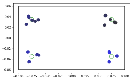
Oops, that was not a good initial guess, as we can see on the overview plot of the force plate. The three scatter clusters in each of the corners are at a substantial distance from the green target points. However, their symmetry lets us hope that this is only due to the non-optimal attempt on the padding parameter.

So let’s tweak this!

With the function above, we iterate all possible values for padding.

padding_candidates = NP.linspace(-0.05, 0.0, 51, endpoint = True)
distances = [PointGroupwiseDistance(data, pad) for pad in padding_candidates]

MPP.plot(padding_candidates, distances, 'k-');

png

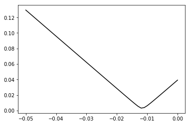
Looks like there is a putative winner:

padding_winner = padding_candidates[NP.argmin(distances)]
print(padding_winner)

-0.012000000000000004

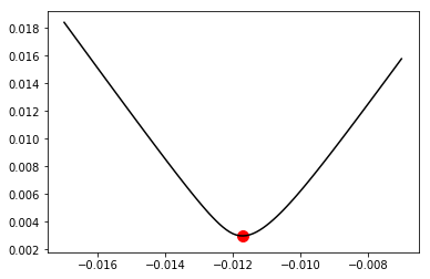
Let’s zoom in even further:

padding_candidates = NP.linspace(padding_winner-0.005, padding_winner+0.005, 101, endpoint = True)
distances = [PointGroupwiseDistance(data, pad) for pad in padding_candidates]
padding_winner = padding_candidates[NP.argmin(distances)]

MPP.plot(padding_candidates, distances, 'k-');
MPP.scatter(padding_winner, NP.min(distances), s = 100, color = 'r', marker = 'o');
padding_winner

-0.011700000000000004

png

# substituting this once more
fp_dimensions = [(qj[0], 0.035), (qj[1], 0.075), (pj[2], padding_winner)]

# generate conversion functions
ComponentsToParameters = { str(param): \
                          SYM.lambdify(force_components, eqn.subs(fp_dimensions), "numpy") \
                      for param, eqn in all_solutions.items()\
                     }

data_vectors = [data.loc[:,col].values for col in rawmeasure_labels]
calculated_values = PD.DataFrame.from_dict({param: eqn(*data_vectors) for param, eqn in ComponentsToParameters.items()})


cm = 1/2.54
figwidth = 18 * cm
figheight = 24 * cm
fig = MPP.figure( figsize = (figwidth, figheight) \
                , facecolor = None \
                )
ax = fig.add_subplot(1,1,1, aspect = 1.)

leg_pos = NP.concatenate([leg_positions[:,:], [leg_positions[0,:]]], axis = 0)
ax.plot(  leg_pos[:,1] * 0.10 \
                    , leg_pos[:,0] * 0.06 \
                    , 'k-')

target_x = [data.loc[data['pt_nr'].values == pt, 'target_px'].values.mean() \
           for pt in NP.unique(data['pt_nr'])]
target_y = [data.loc[data['pt_nr'].values == pt, 'target_py'].values.mean() \
           for pt in NP.unique(data['pt_nr'])]
ax.scatter( target_y \
           , target_x \
           , s = 200 \
           , marker = 'o' \
           , edgecolor = (0.2, 0.6, 0.2) \
           , facecolor = 'none' \
           , label = 'target CoP' \
          )

symbs = {'spread': '^' \
        , 'reference': 'x' \
        , 'loaded': 'v' \
        }
for idx, row in calculated_values.iterrows():
    ax.scatter( row['p_{y}'] \
               , row['p_{x}'] \
               , s = 80 \
               , marker = 'o' \
               , color = (0.2, 0.2, 0.2+0.7*(idx/calculated_values.shape[0])) \
               , label = 'own calculation' \
              )

png

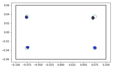
So for this force plate, our padding value turns out to be \(-0.0117\).

I call this procedure “empirical regression” because I did not take the time to wrap the function above into a proper minimizer. This could be done with something from scipy.optimize. However, because we always have visual inspection of the plots, and because the calculation was fast (thanks to lambdify), the process is sufficient for all our purposes.

These were few measurements, and only on four points.

It is worth taking the time to sample a grid of points across the surface of the force plate and use a high number of repetitions. This way you can confirm that the force plate is really isotropic, i.e. all sensors return the same voltage level. You can see that the upper right point is a bit offset, so there might be something wrong there. Or it might just have been a bad measurement. Repetition is key.

Summary

This concludes my series on force plates, by providing the tools to calculate the sensor position below the force plate surface. All it took was a tripod and code we had from the previous posts.

I hope you enjoyed the tour and are now able to understand every aspect of these useful devices.

Comments and feedback are welcome!